This test case suite focuses on the immersed boundary methods applied to the Poisson equation.

This test case suite focuses on the immersed boundary methods applied to the Poisson equation.

This test case suite focuses on the immersed boundary methods applied to the Poisson equation with either Dirichlet or Neumann boundary conditions. The objectives of this test case are:

1. verify the core of the immersed boundary methods.
2. verify the order of spatial convergence of the methods.

For more details, see [1] and [2].

Configurations

Physical domain

The global boundaries are defined by the box:

\begin{align} [-1, +1]^2 &\quad\text{in 2D,} & [-1, +1]^3 &\quad\text{in 3D.} \end{align}

The immersed boundary is either a cylinder or a sphere:

\begin{align} x^2 + y^2 = r_c^2 &\quad\text{(cylinder),} & x^2 + y^2 + z^2 = r_c^2 &\quad\text{(sphere),} \end{align}

where \(r_c = \frac{13}{20}\). The inner domain can be inside or outside the shape. Most cases set the inner domain outside.

Solutions

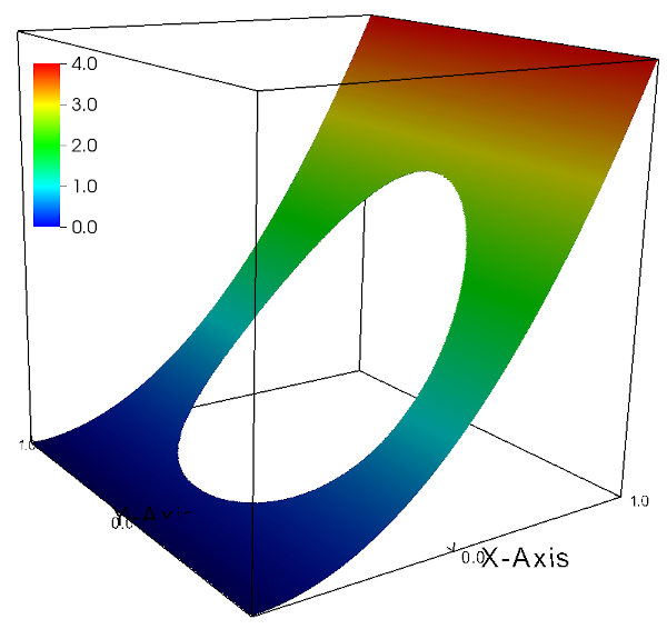
For the parabolic solution, the source term and the boundary conditions are chosen to obtain the following solution (see figure 1):

\begin{align} T(x,y,z) = (1 + x)^2 \end{align}

In the inner domain, the source term is then

\begin{align} S(x,y,z) = 2. \end{align}

The average temperature can be computed analytically. First the volume of the inner domain must be known:

\begin{align} \begin{aligned} V &= 4 - \pi r_c^2 &&= 2.6726771038583124\ldots\quad\text{2D, outside} \\ V &= \pi r_c^2 &&= 1.3273228961416876\ldots\quad\text{2D, inside} \\ V &= 8 - \tfrac{4}{3}\pi r_c^3 &&= 6.8496534900105374\ldots\quad\text{3D, outside} \end{aligned} \end{align}

The average temperatures are thus obtained by:

\begin{align} V \bar{T} &= 2\int_{-1}^{-r_c}{T(x)^2{\rm d}x} + 2\int_{-r_c}^{+r_c}{1 - \sqrt{r_c^2-x^2}T(x)^2{\rm d}x} + 2\int_{+r_c}^{+1}{T(x)^2{\rm d}x} \quad\text{2D, outside} \\ V \bar{T} &= 2\int_{-r_c}^{+r_c}{\sqrt{r_c^2+x^2}T(x)^2{\rm d}x} \quad\text{2D, inside} \\ V \bar{T} &= 4\int_{-1}^{-r_c}{T(x)^2{\rm d}x} + \int_{-r_c}^{+r_c}{4 - \pi (r_c^2-x^2)T(x)^2{\rm d}x} + 4\int_{+r_c}^{+1}{T(x)^2{\rm d}x} \quad\text{3D, outside} \end{align}

The values are given in the table below.

Figure 1: Elevation of the temperature field

For the trigonometric solution, the source term and the boundary conditions are chosen from the following solution:

\begin{align} T(x,y,z) = sin(\pi x) cos(2\times \pi y) \end{align}

In the inner domain, the source term is then

\begin{align} S(x,y,z) = -5 \pi^2 sin(\pi x) cos(2 \pi y) \end{align}

Boundary conditions

The global boundary conditions are chosen as follows:

The immersed boundary conditions type are either Dirichlet or Neumann and given by the parabolic or the trigonometric solutions.

Grids

Rectangular cells are used to perform validation tests (2.8 ratio).

Test case list

Runtime parameters

The following common setting are used:

• The temporal and advection terms of the energy equation are deactivated.
• Several IBM methods are used (see [1,2] for details): direct, linear, LGS, LIS, Q, QO, QGS, QGS, QIS, QISS1, QISS1P3, LGSP3.
• Polynomial interpolation of order 2 and 3 are used.

Results

The details results can be found in [1] and [2].

Following table summarizes the maximum stencil sizes and order of convergences of the various proposed methods for Dirichlet IBCs for parabolic and trigonometric analytical solutions for the 2D and 3D Poisson problems.

Folinwg table summarizes the maximum stencil sizes and order of convergences of the various proposed methods for Neumann IBCs for parabolic and trigonometric analytical solutions for the 2D and 3D Poisson problems.

References

[1] J. Picot, S. Glockner, Discretization stencil reduction of direct forcing immersed boundary methods on rectangular cells: the Ghost Node Shifting Method, Journal of Computational Physics, 364, pp18-48, 2018.

[2] A. M. D. Jost and S. Glockner, Direct forcing immersed boundary methods: Improvements to the Ghost Node Method, Journal of Computational Physics, volume 438, 110371, 2021.