Validation of the flows around circular and elliptic cylinders (2D).

Configuration

The following numerical simulations validate second order immersed boundary method on stationary ﬂows around two cylinders of diﬀerent shapes: circular and elliptic (see [1] for more details). The former has been extensively studied in the literature, while the latter highlights the advantages of rectangular cells and improvements to the direct and ghost-cell methods proposed in [1].

The circular cylinder has diameter \(d=1\); the elliptic cylinder has major axis \(d=1\) and axis ratio \(0.2\); thus the characteristic length is \(d\) for both cylinders. The major axis of the elliptic cylinder is rotated by \(\alpha\) with respect to the original coordinate frame. The angle \(\alpha\) is also the angle of incidence; it is set to \(80°\) for the elliptical cylinder. Figure 1 shows both cylinders with a description of their dimensions.

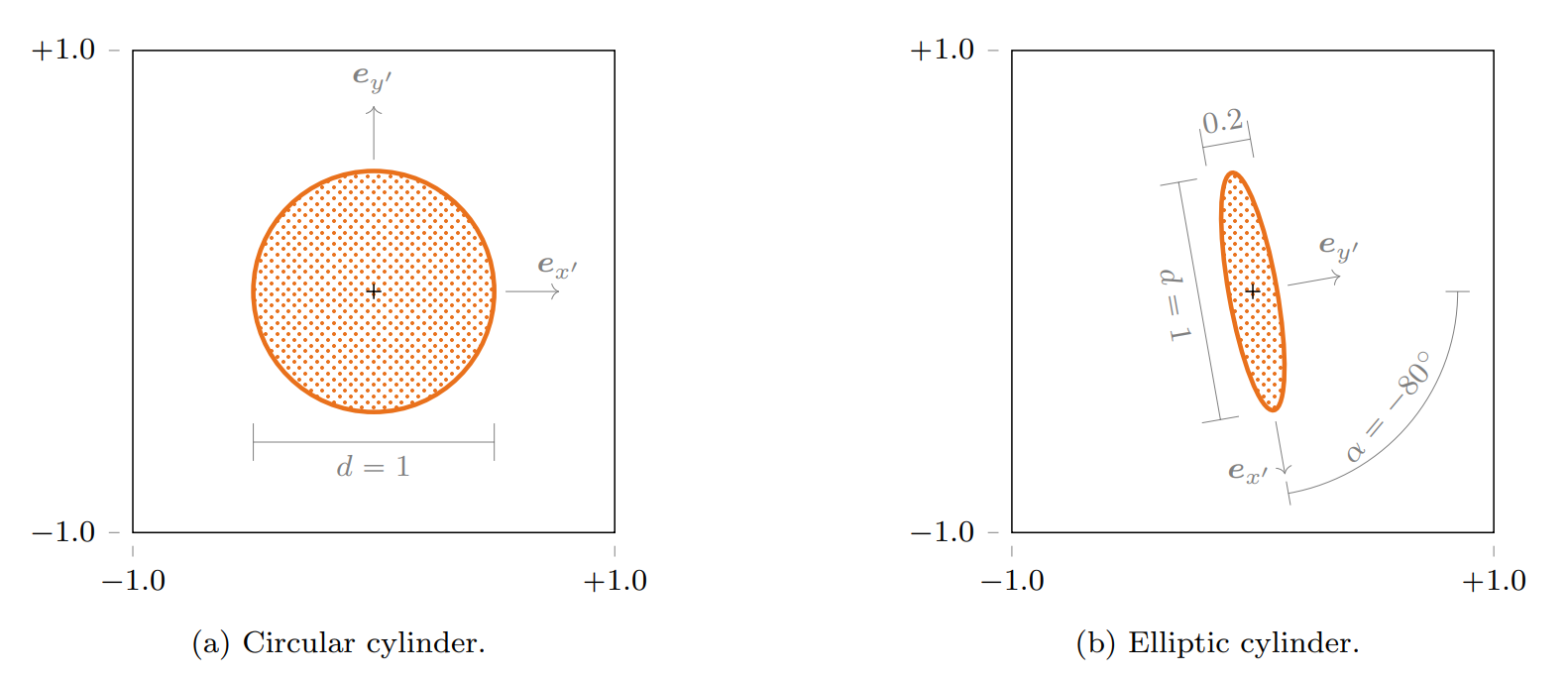
Figure 1: Dimensions of circular and elliptic cylinders.

We choose the free-stream velocity \(u_\infty=1\), and we set the viscosity according to the desired value of the Reynolds number \(Re=d u_\infty / \nu\). For the elliptic cylinder, the Reynolds number is based on the long axis. The Reynolds number is set to \(Re=40\) for the circular cylinder, and set to \(Re=20\) for the elliptic cylinder.

Runtime parameters

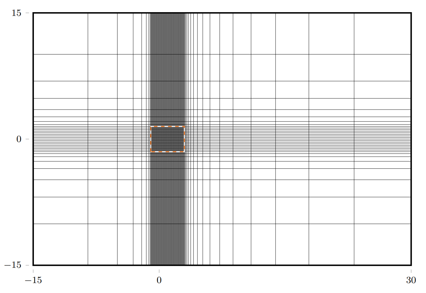
The computational domain represents a tank of the 2-dimensional real space, whose dimensions are \(\Omega = [-15,+30] \times [-15, +15]\), and the ﬂow goes from left to right. Domain boundary conditions are: uniform inlet of velocity \((u_\inf, 0)^T\) at the left boundary, slip at top and bottom boundaries, and Neumann at the right boundary. The cylinder is placed at the origin. A regular grid of ratio \(a=3.0\) is placed over a small domain of interest, of dimensions \([-1,+3] \times [-1.5, +1.5]\), while exponential grids are placed around. On the y-axis, we used that 512 cells in the domain of interest and 256 cells in each exponential region. On the x-axis, we used 1536 cells in the domain of interest to have a=3.0 and 768 cells in each stretched region. Figure 2 shows the computational domain, the grid and the domain of interest.

Figure 2: Computational domain and grid used to simulate the flow around the two cylinders. Only one grid line out of 16 is drawn for the sake of readability.

Second order implicit centered schemes are used. We focus on the direct and the ghost-cell image point linear square shift immersed boundary methods (LIS) [1].

Test case list

Label
cylinder_2D.nts
ellipse_2D.nts

Results

As no analytical solution exists, we compare our results to experimental and numerical data found in the literature. Both direct and linear methods gives very similar results. First, we compare the position of seven different points of interest: four separation points on the surface of the obstacle \(a^-, a^+, b^-, b^+\) and \(d\); two vortex cores \(c^-, c^+\), and the steady point at the right of the wake vortices \(d\). Next figure shows these points for the two cylinders.

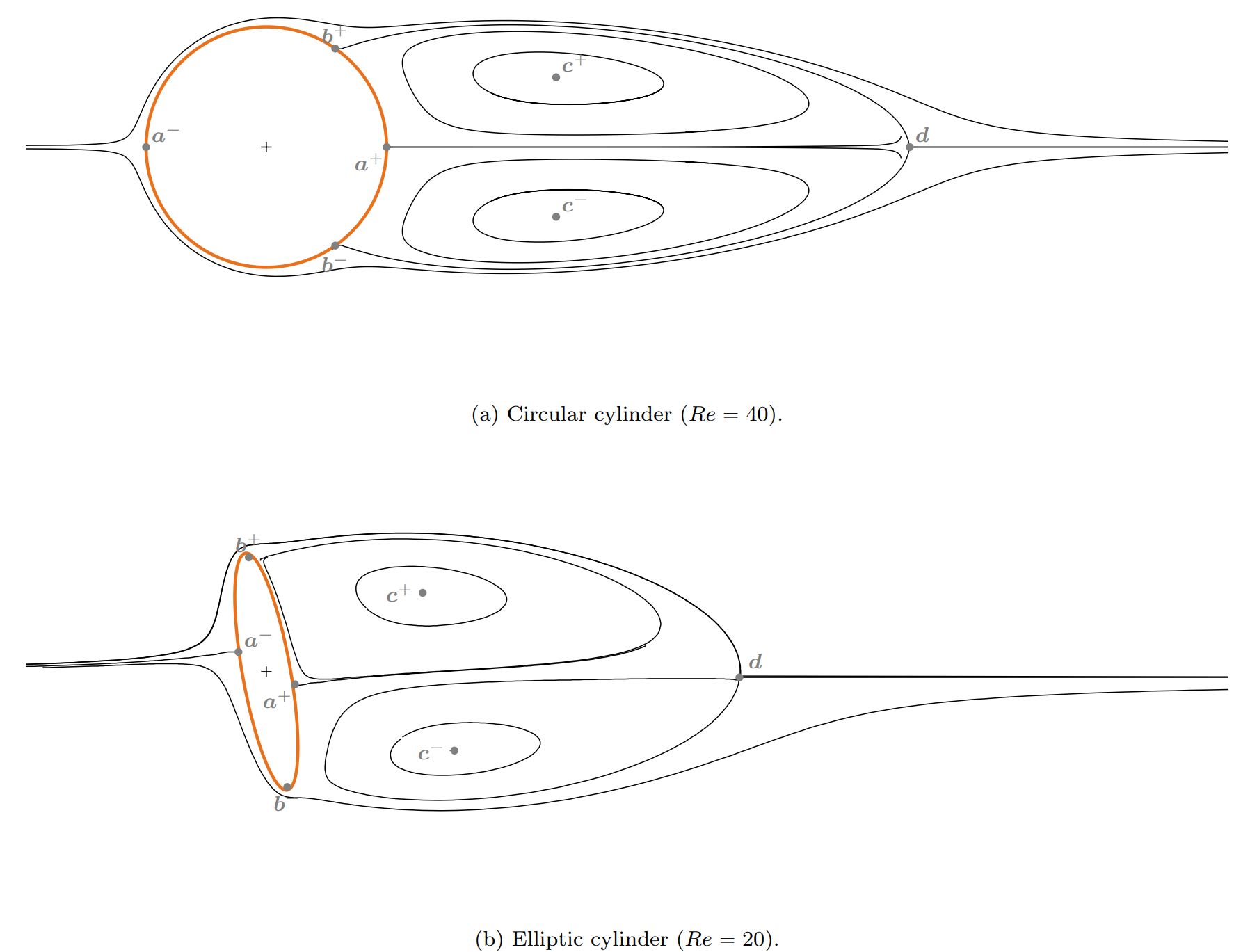
Figure 3: Points of interest of the steady wake flow. The streamlines are extracted from computations.

Coordinates of the points of interest are reported in the two next tables for the circular cylinder and for the elliptic cylinder. Good agreement with literature data is observed for the circular cylinder. Lengths for the elliptic cylinder are coherent with the streamline visualizations of Yoon et al. [2].

Data source	\(λ\)	\(l/d\)	\(a/d\)	\(b/d \)	\(θ/°\)
Coutanceau [3]	0.024	2.04	0.73	0.58	—
	0	2.13	0.76	0.59	53.5
Linnick [4]	0.023	2.28	0.72	0.60	53.6
Calhoun [5]	—	2.18	—	—	54.2
Le [6]	—	2.22	—	—	53.6
Taira [7]	1/60	2.30	0.73	0.60	53.7
Berthelsen [8]	—	2.29	0.72	0.60	53.9
present (direct/linear method)	1/30	2.27	0.72	0.59	53.1

\(𝒂^-/d\)	\(𝒂^+/d\)	\(b^{-}_θ\)/°	\(b^{+}_θ\)/°	\(𝒄^{-}/d\)	\(𝒄^{+}/d\)	\(𝒅/d\)
(-0.11, 0.082)	(0.11, -0.06)	0.3	178.7	(0.782, -0.33)	(0.650, 0.33)	(1.97, -0.02)

Next, we compute the drag and lift coefficients, reported in next table for the circular cylinder (lift coefficients are below \(10^{-8}\)). The value is in the range of values found in the literature.

Data source	\(C_{D_p}\)	\(C_{D_ν}\)	\(C_D\)
Tritton [9]			1.57
Linnick [4]			1.54
Calhoun [5]			1.62
Le [6]			1.56
Taira [7]			1.54
Berthelsen [8]			1.59
present (direct/linear method)	1.026	0.533	1.559

Drag and Lift coefficients are reported in next table for the elliptic cylinder, along with values obtained in the literature. Values are also in the range of values found in the literature. Most of the drag is due to the pressure drag. It is interesting to note that pressure and viscosity have opposite contribution to lift.

Data source	\(C_{D_p}\)	\(C_{D_ν}\)	\(C_D\)	\(C_{L_p}\)	\(C_{L_ν}\)	\(C_L\)
D'alessio [10]			2.116			0.256
Dennis [11]			2.089			0.255
Yoon [2]			2.102			0.252
present (direct/linear method)	1.864	0.266	2.130	0.303	-0.057	0.246

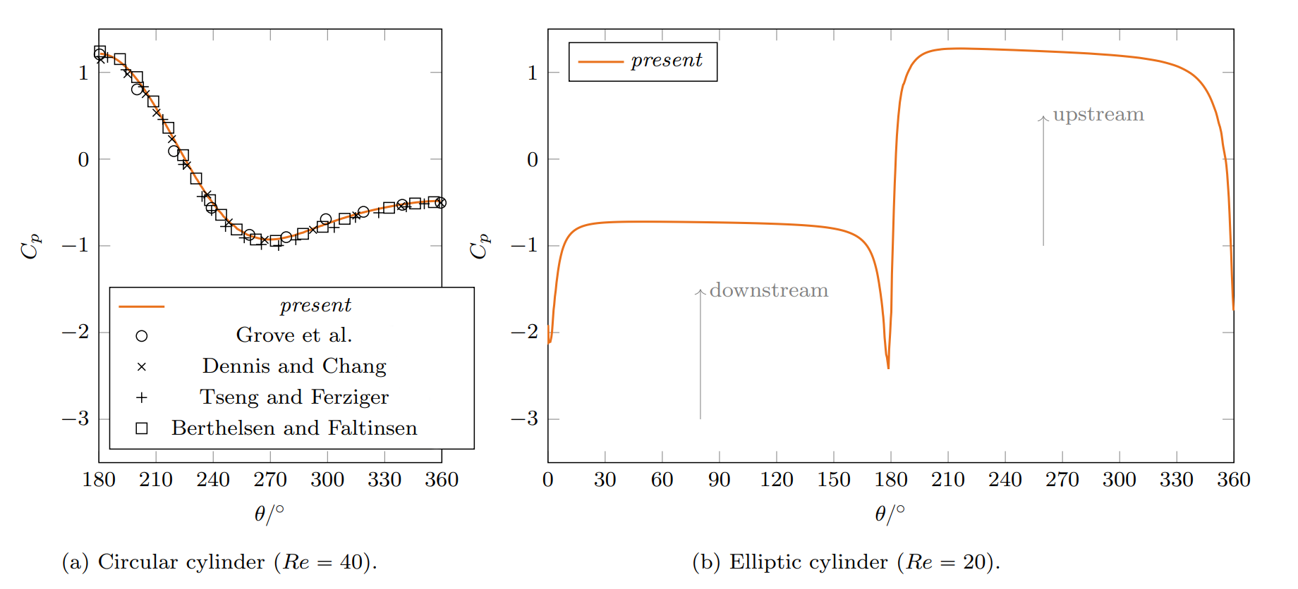
Finally, profiles of normalized pressure Cp as a function of θ are shown on next figure. The profile for the circular cylinder follows closely the profiles found in the literature [8,12,13,14]. The profile for the elliptic cylinder has a maximum and minimum pressure than the circular cylinder. Although, very low pressure are seen at the tips of the ellipse ( \(θ=0°, 180°\)).

Figure 4: Normalized pressure profile Cp around the cylinders.

References

[1] J. Picot, S. Glockner, Discretization stencil reduction of direct forcing immersed boundary methods on rectangular cells: the Ghost Node Shifting Method, Journal of Computational Physics, 364, pp18-48, 2018.

[2] H. S. Yoon, J. Yin, C. Choi, S. Balachandar, M. Y. Ha, Bifurcation of laminar flow around an elliptic cylinder at incidence for low Reynolds numbers, Progress in Computational Fluid Dynamics, an International Journal 16 (3) (2016) 163–178.

[3] M. Coutanceau, R. Bouard, Experimental determination of the main features of the viscous flow in the wake of a circular cylinder in uniform translation. Part 2. Unsteady flow, Journal of Fluid Mechanics 79 (2) (1977) 257–272, 0022-1120, doi:10.1017/S0022112077000147.

[4] M. N. Linnick, H. F. Fasel, A high-order immersed interface method for simulating unsteady incompressible flows on irregular domains, Journal of Computational Physics 204 (1) (2005) 157–192, doi:10.1016/j.jcp.2004.09.017.

[5] D. Calhoun, A Cartesian Grid Method for Solving the Two-Dimensional Streamfunction-Vorticity Equations in Irregular Regions, Journal of Computational Physics 176 (2) (2002) 231–275, doi:10.1006/jcph.2001.6970.

[6] D. Le, B. Khoo, J. Peraire, An immersed interface method for viscous incompressible flows involving rigid and flexible boundaries, Journal of Computational Physics 220 (1) (2006) 109–138, doi:10.1016/j.jcp.2006.05.004.

[7] K. Taira, T. Colonius, The immersed boundary method: A projection approach, Journal of Computational Physics 225 (2) (2007) 2118–2137, doi:10.1016/j.jcp.2007.03.005.

[8] P. A. Berthelsen, O. M. Faltinsen, A local directional ghost cell approach for incompressible viscous flow problems with irregular boundaries, Journal of Computational Physics 227 (9) (2008) 4354–4397, doi:10.1016/j.jcp.2007.12.022.

[9] D. J. Tritton, Experiments on the flow past a circular cylinder at low Reynolds numbers, Journal of Fluid Mechanics 6 (04) (1959) 547, 1469-7645, doi:10.1017/S0022112059000829.

[10] S. J. D. D’alessio, S. C. R. Dennis, A vorticity model for viscous flow past a cylinder, Computers & fluids 23 (2) (1994) 279–293.

[11] S. C. R. Dennis, P. J. S. Young, Steady flow past an elliptic cylinder inclined to the stream, Journal of engineering mathematics 47 (2) (2003) 101–120.

[12] A. S. Grove, F. H. Shair, E. E. Petersen, An experimental investigation of the steady separated flow past a circular cylinder, Journal of Fluid Mechanics 19 (1) (1964) 60, 1469-7645, doi:10.1017/S0022112064000544.

[13] S. C. R. Dennis, G.-Z. Chang, Numerical solutions for steady flow past a circular cylinder at Reynolds numbers up to 100, Journal of Fluid Mechanics 42 (03) (1970) 471, 1469-7645, doi:10.1017/S0022112070001428.

[14] Y.-H. Tseng, J. H. Ferziger, A ghost-cell immersed boundary method for flow in complex geometry, Journal of Computational Physics 192 (2) (2003) 593–623, doi:10.1016/j.jcp.2003.07.024.