|
|
0.6.0
|
|
|
0.6.0
|
Validation of the lid driven cavity flows with stationary and rotating immersed cylinders (2D)
Validation of the lid driven cavity flows with stationary and rotating immersed cylinders (2D)
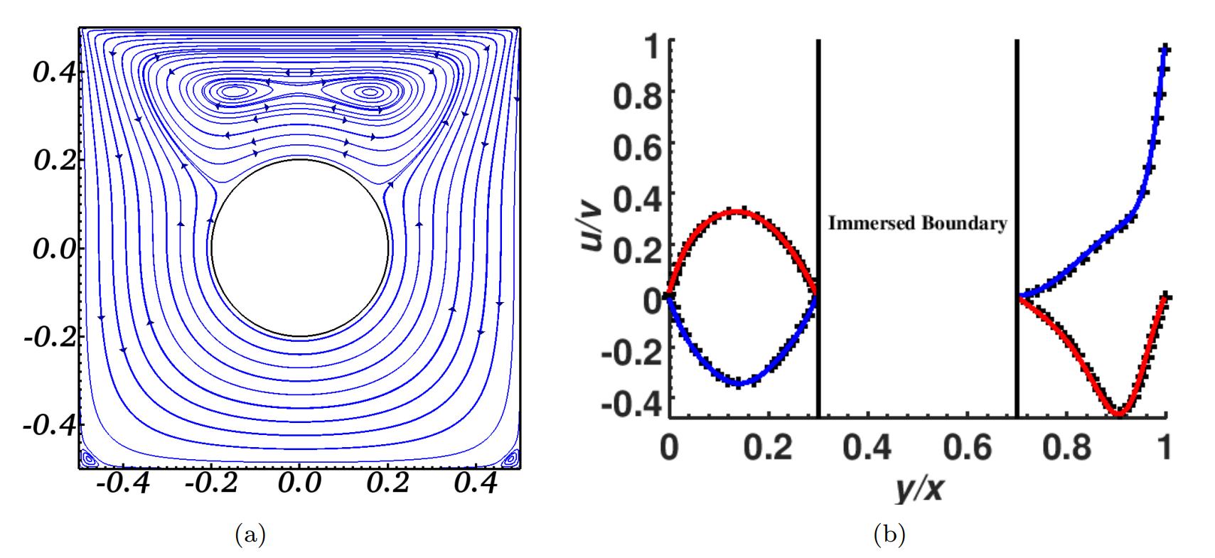
The first validation case is the lid-driven cavity with a stationary immersed cylinder case proposed by Cai et al. [3]. A circular cylinder at \(Re=1000\) with a diameter \(D=0.4L\) is placed in the middle of a square cavity with side length \(L=1\). The following numerical simulations validate second order immersed boundary methods [1,2].
The boundary conditions for the domain boundaries for velocity are uniform flow \(u=(1.0,0.0)\) for the top wall and no-slip boundary conditions for the remaining boundary, while pressure increment has zero normal gradient for all domain boundaries.
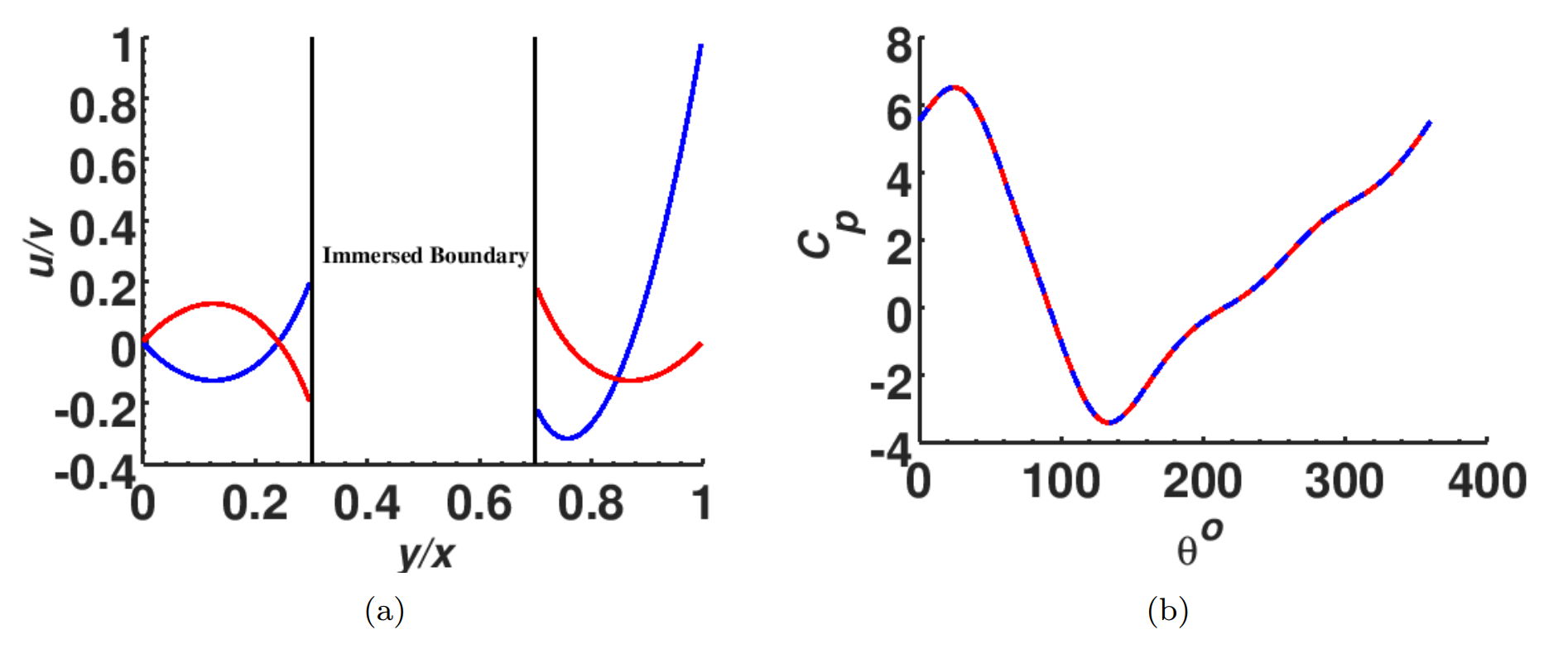
A lid-driven cavity with a rotating immersed boundary is also considered as a second validation test case. The numerical setup is identical to that for a stationary immersed boundary except for the angular velocity \(ω=1\) rad of the circular cylinder and \(Re=5\).
A regular grid size \(N^2=256^2\) is used. Implicit discretization and the second order centered advection scheme are used. For the stationary cylinder case, we focus on ghost-cell linear immersed boundary methods with image shift approach (LIS). For the rotating cylinder test case, we focus on the linear (L), quadratic QSS1 and linear ghost shift method (LGS).
Figure 1 shows the good agreement between the current u and v-velocity profiles along the y and x-direction centerline, respectively, for the LIS method with those of Cai et al. [3].
For the rotating cylinder case, Figure 2a shows the current u and v-velocity profiles along the y and x-direction centerline, respectively, and Figure 2b shows the distribution of the coefficient of pressure, as a function of θ, along the surface of the circular cylinder for the L and QISS1 with third-order Lagrange interpolation (p=3) methods. It should be noted that the reduced stencil size of 1 of LIS methods, compared to the stencil size of 2 of the L method, results in similar results as those presented in Figure 2.
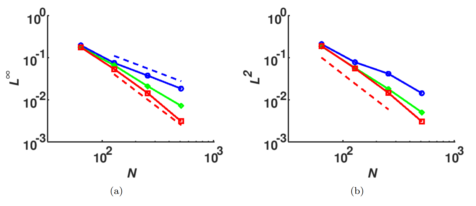
To further highlight the improvements in accuracy and convergence order of the proposed LGS and QISS1 with \(p=3\) whilst maintaining the same stencil size of 2 as the L method, the \(L_\infty\) and \(L^2\) error norms of pressure are considered. As the current validation test case does not have an exact solution, the results obtained on a highly resolved grid \(N^2=512^2\) are used as the baseline when computing the error norms. The errors norms of velocity u are not currently considered as the Dirichlet IBCs guarantee a second-order convergence as seen in Section 6.1. Figure 3 shows the \(L_\infty\) and \(L^2\) error norms of pressure for the L method and, as expected, display first and in-between first and 1.5 order convergence, respectively. The results of the currently proposed LGS and QISS1 with p=3 display an improved order of convergence and are significantly more accurate than those obtained with the L method. The LGS method with \(p=3\) has a 1.5 and second order convergence for the \(L_\infty\) and \(L^2\) error norms, respectively, while the QISS1 with \(p=3\) displays a second-order convergence for both error norms.
[1] J. Picot, S. Glockner, Discretization stencil reduction of direct forcing immersed boundary methods on rectangular cells: the Ghost Node Shifting Method, Journal of Computational Physics, 364, pp18-48, 2018.
[2] A. M. D. Jost and S. Glockner, Direct forcing immersed boundary methods: Improvements to the Ghost Node Method, Journal of Computational Physics, volume 438, 110371, 2021.
[3] S.-G. Cai, A. Ouahsine, J. Favier, and Y. Hoarau, “Moving immersed boundary method,” International Journal for Numerical Methods in Fluids, vol. 85, no. 5, pp. 288–323, 2017.