|
|
0.6.0
|
|
|
0.6.0
|
VOF-PLIC test case of single vortex (2D)
VOF-PLIC test case of single vortex (2D)
This test case solves advection of a disc of fluid in a sheared analytical velocity field. It is interesting because of the large variation of the interface topology. It is particularly adapted to measure mass-conservation. The objective is to compare two VOF-PLIC (Piecewise Linear Interface Construction) advection methods, the conservative method presented in [1] and the non conservative one presented in [2].
The simulation takes place in a 2D box of coordinates \( (0,0) \) and \( (1,1) \). This domain is discretized uniformly with N cells in each directions. A bubble of fluid A is initialized in a domain full of fluid B. The coordinates of the center of the bubble at initial time is \( (0.5,0.75) \) with a \( 0.15m \) radius. The simulation runs during \( T=1.5s \).
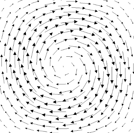
The velocity field is inverted at time \( t=T/2 \) such a way to obtain ideally a final state equal to the initial state.
| Time t[s] | \(u(x,y)\) | \(v(x,y)\) |
|---|---|---|
| \( t<0.75s \) | \( 2sin^2(\pi x)cos(\pi y)sin(\pi y) \) | \(-2cos(\pi x)sin(\pi x)sin^2(\pi y)\) |
| \( t>0.75s \) | \( -2sin^2(\pi x)cos(\pi y)sin(\pi y) \) | \(2cos(\pi x)sin(\pi x)sin^2(\pi y)\) |
To ensure that CFL of the method is always respected, we set a time step \( \Delta t \) such as
\begin{align} \Delta t = \frac{0.2}{N} \end{align}
Below is shown some plots of the simulation with various \( (N,N) \) grids.
![Figure 2 : Isocontour of the volume fraction value 0.5, non-conservative method (red), conservative method (blue), initial configuration (black), N = 32] (single_vortex_32.png) ![Figure 3 : Isocontour of the volume fraction value 0.5, non-conservative method (red), conservative method (blue), initial configuration (black), N = 64] (single_vortex_64.png) ![Figure 4 : Isocontour of the volume fraction value 0.5, non-conservative method (red), conservative method (blue), initial configuration (black), N = 128] (single_vortex_128.png) ![Figure 5 : Isocontour of the volume fraction value 0.5, non-conservative method (red), conservative method (blue), initial configuration (black), N = 256] (single_vortex_256.png)
Isocontour of conservative and non-conservative methods are nearly surimpose. From N=64, the precision of the reconstruction become qualitatively acceptable for both methods at time t=T. The bubble returns to its original point with a slight difference compared to the initial configuration (black bubble). Moreover, at time t=1.5s, since N=128, we don't observe formation of secondary bubbles. Increasing the precision of the grid improves the description of the interface, the tail become more slender and the nose moves closer to the center of the domain.
![Figure 6 : Isocontour of the volume fraction value 0.5 for consevative method, in red N=64, in green N=128 and in blue N=256] (single_vortex_2D_comparison.png)
In order to evaluate mass loss \( \varepsilon \) during the simulation, we compute the difference between the volume fraction of fluid at initial time and at time T.
\begin{align} \varepsilon = \sum \limits^{N^2}_{i=1}f_i - \sum \limits^{N^2}_{i=1} f_i^0 \end{align}
To evaluate mesh convergence, we define the \( L_1 \) norm of the difference between the initial and the current volume fraction as:
\begin{align} L_1 = \sum \limits^{N^3}_{i=1} |f_i - f^0_i| \\ \end{align}
We also compute local convergence order \( p \) of the method evaluating the evolution of the error with the mesh refinement:
\begin{align} p = \frac{ln\left( \frac{E_2}{E_1} \right)}{ln\left (\frac{N_1}{N_2} \right)} \end{align}
where \( E_1 \) and \(E_2 \) are error for mesh 1 and mesh 2, of size \( N_1\) and \(N_2\) respectively.
The following tables show for different spatial discretization the material loss for the two different advection methods.
\begin{align} \textbf{Non-conservative method} \end{align}
| Grid size N | \( \Delta x \) | \( \varepsilon_{air}\) (non conservative method) | \( L_1 \) | p |
|---|---|---|---|---|
| 16 | 1/16 | \( -2.42 \times 10^{-3}\) | \( 1.84 \times 10^{-2}\) | |
| 32 | 1/32 | \( -1.24 \times 10^{-3} \) | \( 8.19 \times 10^{-3}\) | \(1.16 \) |
| 64 | 1/64 | \( -6.57 \times 10^{-4} \) | \( 3.09 \times 10^{-3}\) | \(1.40 \) |
| 128 | 1/128 | \( -3.31 \times 10^{-4} \) | \( 1.40 \times 10^{-3}\) | \(1.14 \) |
| 256 | 1/256 | \( -1.65 \times 10^{-4} \) | \( 8.12 \times 10^{-4}\) | \(0.78 \) |
| 512 | 1/512 | \( -8.32 \times 10^{-5} \) | \( 4.05 \times 10^{-4}\) | \(1.00 \) |
| 1024 | 1/1024 | \( -4.17 \times 10^{-5} \) | \( 1.63 \times 10^{-4}\) | \(1.31 \) |
\begin{align} \textbf{Conservative method} \end{align}
| Grid size N | \( \Delta x \) | \( \varepsilon_{air}\) (conservative method) | \( L_1 \) | p |
|---|---|---|---|---|
| 16 | 1/16 | \( 1.11 \times 10^{-16} \) | \( 1.50 \times 10^{-2}\) | |
| 32 | 1/32 | \( 4.44 \times 10^{-16} \) | \( 4.98 \times 10^{-3}\) | \(1.59 \) |
| 64 | 1/64 | \( 0.0 \) | \( 3.56 \times 10^{-3}\) | \(0.48 \) |
| 128 | 1/128 | \( 0.0 \) | \( 1.67 \times 10^{-3}\) | \(1.09 \) |
| 256 | 1/256 | \( 2.22 \times 10^{-16} \) | \( 4.06 \times 10^{-4}\) | \(2.04 \) |
| 512 | 1/512 | \( 0.0 \) | \( 2.01 \times 10^{-4}\) | \(1.01 \) |
| 1024 | 1/1024 | \( 1.11 \times 10^{-16} \) | \( 2.07 \times 10^{-4}\) | \(-0.04 \) |
Results confirm that even though the method presented in [2] shows pretty good results concerning mass conservation, the one presented in [1] is fully conservative (up to machine precision). In constrast, the convergence order of the non conservative method is more stable than the one of the conservative method and is near to one. Moreover, nearly same errors are noticed.
[1] G.D. Weymouth, Dick K.-P. Yue, Conservative Volume-of-Fluid method for free-surface simulations on Cartesian-grids, Journal of Computational Physics 229 (2010) 2853–2865
[2] Jérôme Breil. Modélisation du remplissage en propergol de moteur a propulsion solide. Mécanique des fluides [physics.class-ph]. Université de Bordeaux 1, 2001. Français. tel-0147869. https://tel.archives-ouvertes.fr/tel-01478691