Description of the test case

This test case solves the problem of a rising bubble under gravity entrainment [1]. It consists of two immiscible fluids separated by an interface.

This problem involves the following numerical methods:

Navier-Stokes solver
Bi-phasic interface transport
Surface tension force computation

This test case aims at the validation of the conservative VOF-PLIC method [2].

The validation criteria are:

The position and velocity of the center of mass of the bubble
The geometry of the bubble
The machine precision mass conservation

Configuration

Physical domain and geometry

The simulations take places in a 2D box of fluid of coordinates \((0,0)\) and \((1,2)\). The bubble is centered at the position \((0.5,0.5)\) and is of radius \(0.25 m\).

Fluids' properties

The first fluid is the denser one that surrounds the bubble (noted with \(2\) as a subscript). There are two different cases:

Case	\(\rho_1\)	\(\rho_2\)	\(\mu_1\)	\(\mu_2\)	\(\sigma\)
A	1000	100	10	1	24.5
B	1000	1	10	0.1	1.96

where \(\sigma=\sigma_{1,2}\) is the surface tension coefficient between the two fluids.

Initial and boundary conditions

The initial velocity is null in the whole domain.

We have used the same boundary conditions as in the literature [1]. The left and right boundary conditions are slip; the bottom and top boundary conditions are null velocity (wall).

Other elements

The gravity is set to \(g=0.98 m.s^{-2}\) in the \(y\) direction, as in the literature. The problem is studied until \(t=3s\) with a \(0.001s\) time step to verify the CFL.

In order to evaluate mass loss \( \varepsilon \) during the simulation, we compute the difference between the volume fraction of fluid at initial time and at time T.

\begin{align} \varepsilon = \sum \limits^{N^2}_{i=1}f_i - \sum \limits^{N^2}_{i=1} f_i^0 \end{align}

Runtime parameters

In the .nts files : CASE variable is used to choose between the two cases and the h variable defines cell size in all directions.

Results

Test case A

The following figure shows comparison of the volume fraction isocontour at time t=3s between 1/40 and 1/320 mesh size.

Figure 1: Isocontour of volume fraction 0.5 at time t=3s for test case A in blue h=1/320 and in red h=1/40

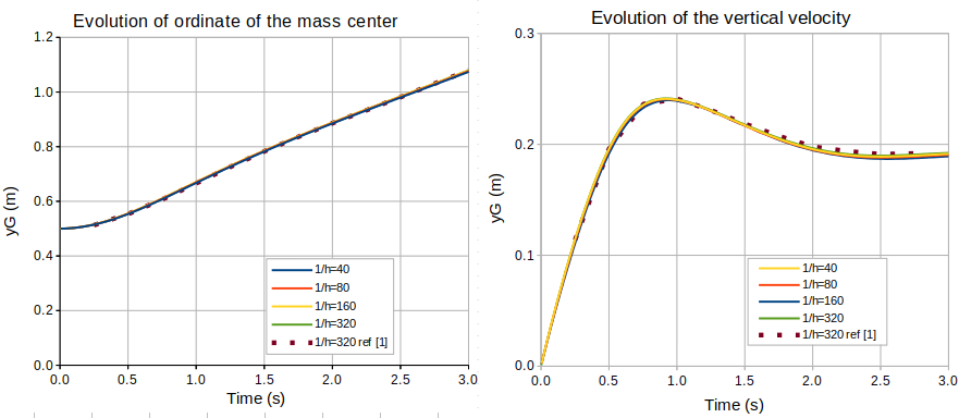
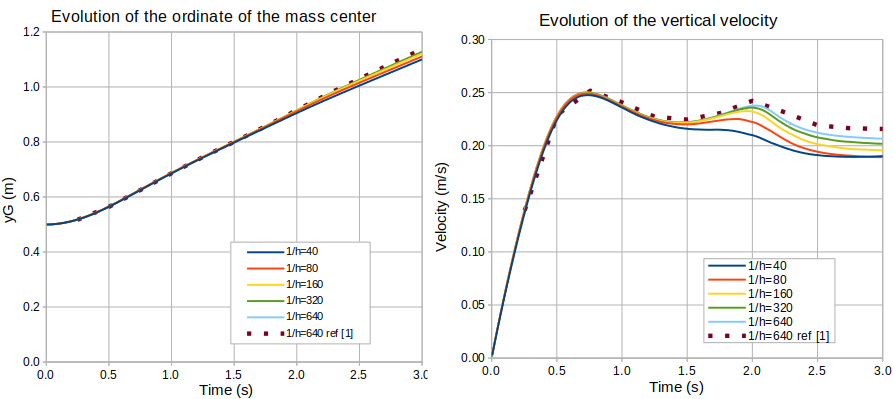
In order to complete the validation we compare in the following plots the reference evolution of the center of mass position and velocity presented in [2], with the computed evolution.

Figure 2: Velocity and position of the bubble mass center

Next table shows the mass conservation results:

Grid size h	\( \varepsilon \)
1/40	\( 4.44 \times 10^{-16} \)
1/80	\( 1.33 \times 10^{-15} \)
1/160	\( 1.42 \times 10^{-14} \)
1/320	\( 4.44 \times 10^{-16} \)

Test case B

The following figure shows comparison of the volume fraction isocontour at time t=3s between 1/40 and 1/320 mesh size.

Figure 3: Isocontour of volume fraction 0.5 at time t=3s for test case A in blue h=1/320 and in red h=1/40

In order to complete the validation we compare in the following plots the reference evolution of the center of mass position and velocity presented in [2], with the computed evolution.

Figure 4: Velocity and position of the bubble mass center

Next table shows the mass conservation results:

Grid size h	\( \varepsilon \)
1/40	\( 1.78 \times 10^{-15} \)
1/80	\( 8.88 \times 10^{-16} \)
1/160	\( -4.44 \times 10^{-16} \)
1/320	\( 2.26 \times 10^{-14} \)
1/640	\( 2.66 \times 10^{-15} \)

References

[1] S. Hysing, S. Turek, D. Kuzmin, N. Parolini, E. Burman, S. Ganesan, L. Tobiska, Quantitative benchmark computations of two-dimensional bubble dynamics, International Journal for Numerical Methods in Fluids 60 (11) (2009) 1259–1288.

[2] G.D. Weymouth Conservative Volume-of-Fluid method for free surface simulations on Cartesian-grids, Journal of Computational Physics 229 (2010) 2853-2865.