The technique known as the method of manufactured solutions involves the development of an a priori known analytical solutions for the governing equations. The procedure introduces modifications of the original equations by adding source term on the right-hand side of equations. These source terms are considered as input, for reproducing the manufactured solution.

In literature, few manufactured solutions for compressible subsonic flows have been developed to validate novel algorithms. After a detailed analysis of the nature and properties of already proposed solutions, we proposed in [1] the following generic, well posed, and reproducible manufactured solution of the two-dimensional compressible Navier-Stokes for a perfect gas in a square domain \(\Omega=[0,1]\times[0,1]\) where the pressure \(p(x,y,t)\), the temperature \(T(x,y,t)\), the density \(\rho(x,y,t)\) and the velocity \(\mathbf{u}=(u,v)^T\) read to

\[ p = p_0 + p_1\sin(\pi y) \sin(\pi x) \cos(2\pi f t), \]

\[ T = T_0 + T_1 \sin(\pi y) \cos(\pi x) \cos(2\pi f t), \]

\[ \rho = p \big/ R T, \]

\[ u = u_0 \sin^2(\pi x) \sin(2 \pi y) \cos(2\pi f t); \]

\[ v = u_0 \sin(2\pi x)\sin^2(\pi y) \cos(2\pi f t); \]

with \(f\) the frequency in \(Hz\), \(p_0\) and \(p_1\) the reference and fluctuation pressure in \(Pa\), \(T_0\) and \(T_1\) the reference and fluctuation temperature \(K\), \(u_0\) the reference velocity in \(ms^{-1}\) and \(R\) the universal gas constant in \(JK^{-1}kg^{-1}\). The perfect gas EoS permits the verification of the solver with time- and space-dependent material properties, except for dynamic viscosity and conductivity considered as constant here. and \(\mu\) the viscosity.

One notices good properties of the solution to simulate a subsonic flow with incremental pressure correction method as the non-zero pressure gradient at boundary or the non-zero divergence field. Time-dependent Dirichlet boundary conditions are applied for temperature fields. For velocity boundary conditions, all the boundaries have no-slip conditions while Neumann homogeneous boundary condition is imposed on pressure increment.

To investigate the accuracy of the resolved fields and different ranges of dimensionless parameters, three specific manufactured solutions are introduced in the following three subsections by tuning parameters. It is helpful to test the proposed method on low Mach solution as encountered in compressible natural flows (e.g. \(Ma_0 \approx 10{-3}\)), as well on solution with much larger Mach (e.g. \(Ma_0 \approx 0.6\)).

The following parameters will remain constant for all three cases :

\(f=700 Hz\),

\(p_0=10^5 Pa\),

\(p_1=2 \ 10^3 Pa\),

\(T_0=300K\),

\(R=287 JK^{-1}kg^{-1}\),

\(\gamma=1.4\),

\(\mu=1.85 \ 10^{-5} Pas^{-1}\).

All the convergence studies consider the final time \(t_f=2 10^{-3}s\) corresponding more than one and a half times the period \(T=1/f\).

Configurations

Three configuration are investigated.

Isothermal high Mach subsonic manufactured solution

The isothermal flow case considers the following parameters \(T_1=0K\), \(u_0=200 ms^{-1}\). We present this unsteady flow solution for whoever wants to analyse the temporal order without considering the coupling of the Navier–Stokes equations and the energy equation. The dimensionless parameters of this case are \(Re_0 =1.26 \ 10^7\), \(Ma_0 =5.76 \ 10^{-1}\).

Anisothermal high Mach subsonic manufactured solution

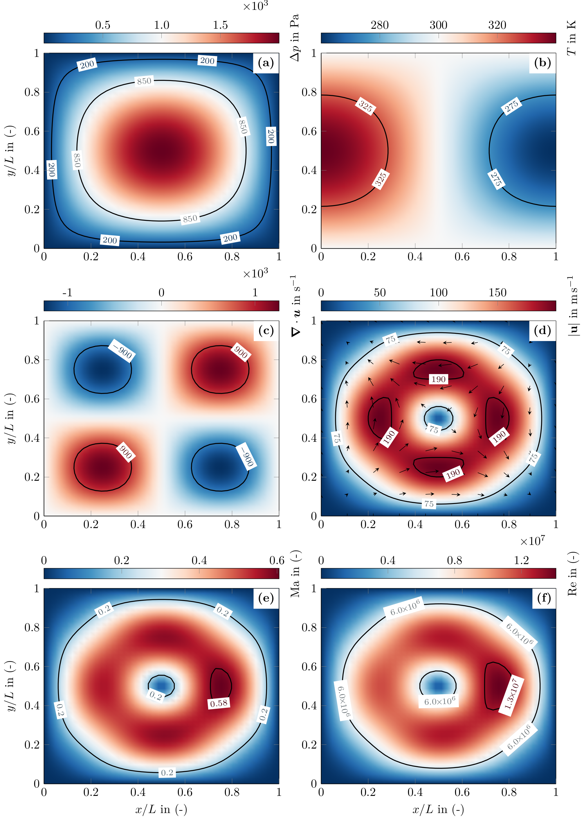
A fully compressible subsonic case is now studied considering the following parameters \(T_1=40K\), \(u_0=200 ms^{-1}\), \(\lambda=10^{-2} Wm^{-1}K^{-1}\). We investigate temporal order of convergence on a test case with the following dimensionless parameters: \(Re_0 = 1.26 \ 10^7\), \(Ma_0 = 5.76 \ 10^{-1}\) and \(Pr_0 = 1.86\).

Firstly, we present next figure the variations of the primitive variables as well as the local variations of Mach and Reynolds numbersof the proposed anisothermal manufactured solution. One may notice strong divergence variations and a maximal local Mach number at \(t=0s\) of 0.6, twice the incompressible limit.

Anisothermal low Mach subsonic manufactured solution

A low Mach fully compressible subsonic case in now studied considering the following parameters \(T_1=40K\), \(u_0=2 ms^{-1}\), \(\lambda=10^{-2} Wm^{-1}K^{-1}\). We investigate spatial and temporal order of convergence on a test case with the following dimensionless parameters: \(Re_0 = 1.26 \ 10^5\), \(Ma_0 = 5.76 \ 10^{-3}\) and \(Pr_0 = 1.86\).

Runtime parameters

Main parameters to run this test case are:

• incremental pressure correction method for subsonic compressible flows
• implicit second order scheme
• HYPRE or MUMPS solvers

Results

Isothermal high Mach subsonic manufactured solution

Next tables present the temporal convergence study. First time step \(\Delta t=2 \ 10^{-4}s\) equal to \(CFL=1.78 \ 10^1\). Mesh size is \(256^2\) and \(t_f=2 \ 10^{-3}s\). Second-order convergence in time is achieved for velocity, pressure, and density, considering both the \(L_2\) and \(L_{\infty}\) norms.

Time step	Velocity L2 error	order	Velocity Linf error	order	Pressure L2 error	order
0.0002	39.31645645984818	n/a	64.41675218615858	n/a	5852.681032029896	n/a
0.0001	14.968262836113222	1.393	25.698133619695767	1.326	1860.9651085834257	1.653
5e-05	4.2894425110243075	1.803	7.930524730416977	1.696	532.5053437090744	1.805
2.5e-05	1.119708325613752	1.938	2.116275666476838	1.906	140.21888023808532	1.925
1.25e-05	0.2881571266375633	1.958	0.5488597118419705	1.947	35.94412423402746	1.964
6.25e-06	0.07738601580989159	1.897	0.14785586561723107	1.892	9.641244185904915	1.898

Time step	Pressure Linf error	order	Density L2 error	order	Density Linf error	order
0.0002	14672.075979975089	n/a	0.06797538945447035	n/a	0.1704073865270046	n/a
0.0001	4934.611105517159	1.572	0.0216139966153708	1.653	0.057312556393927405	1.572
5e-05	1625.09031730759	1.602	0.006184731053531642	1.805	0.018874452001249598	1.602
2.5e-05	438.6641291041774	1.889	0.001628558423206566	1.925	0.005094821476239186	1.889
1.25e-05	113.07448630056356	1.956	0.0004174695032988092	1.964	0.0013132925238161786	1.956
6.25e-06	30.062399102140937	1.911	0.00011197728438913988	1.898	0.0003491567839970511	1.911

Anisothermal high Mach subsonic manufactured solution

We present in next tables the temporal convergence study of the case. First time step \(\Delta t=2 \ 10{-4}s\) equal to \(CFL=1.78 \ 10^1\). Mesh size is \(256^2\) and \(t_f=2 \ 10^{-3}s\). The proposed method reaches the temporal second-order for all the resolved fields, for both \(L_2\) and \(L_{\infty}\) norms.

Time step	Velocity L2 error	order	Velocity Linf error	order	Pressure L2 error	order	Pressure Linf error	order
0.0002	37.527860706252895	n/a	74.55934422916901	n/a	6229.605685362033	n/a	19751.75722022538	n/a
0.0001	13.661037593190175	1.458	24.928980425518436	1.581	1885.1282274790572	1.724	5279.211075896502	1.904
5e-05	3.8736155313864296	1.818	6.912996564784303	1.850	520.029572526077	1.858	1547.909641423432	1.770
2.5e-05	1.0120649212121173	1.936	1.8433466183603855	1.907	135.16697369818706	1.944	401.75603319900114	1.946
1.25e-05	0.260031808726393	1.961	0.48315938417927984	1.932	34.380191005606875	1.975	105.87013056162913	1.924
6.25e-06	0.06917478983598042	1.910	0.1323741578140074	1.868	9.064653411694758	1.923	28.80638265918474	1.878

Time step	Temperature L2 error	order	Temperature Linf error	order	Density L2 error	order	Density Linf error	order
0.0002	7.6155839938693894	n/a	31.533408363838504	n/a	0.054573015250324715	n/a	0.19780350882443187	n/a
0.0001	2.518982595760653	1.596	8.641991549962086	1.867	0.017112939808475384	1.673	0.04451230057087452	2.152
5e-05	0.6835194744834995	1.882	2.402884714440006	1.847	0.0047276928929803315	1.856	0.013850113154384447	1.684
2.5e-05	0.17667470743723276	1.952	0.630403087487764	1.930	0.001234247561890226	1.938	0.004020269741536575	1.785
1.25e-05	0.04528303693453828	1.964	0.16174277888046618	1.963	0.00031592368024915905	1.966	0.0010844959662534848	1.890
6.25e-06	0.012222570399266339	1.889	0.04300378405406491	1.911	8.417979076976992e-05	1.908	0.0003079116504129953	1.816

We also present in next tables the spatial convergence study with a constant Courant number of \(\mathrm{CFL}=1\) for each simulation necessary to attenuate the temporal error. Courant number \(\mathrm{CFL}=1\) and \(t_f=2 \ 10^{-3}s\). Second-order spatial convergence is also confirmed for all fields considering both \(L_2\) and \(L_{\infty}\) norms.

Mesh	Velocity L2 error	order	Velocity Linf error	order	Pressure L2 error	order	Pressure Linf error	order
64x64	3.0546651600907904	n/a	5.712061825056039	n/a	381.11625308926824	n/a	1125.3690481191486	n/a
128x128	0.8000101788214035	1.933	1.517020259074081	1.913	99.12707069358329	1.943	304.0952329990088	1.888
256x256	0.20222805610313174	1.984	0.3910632099537641	1.956	24.935299726185107	1.991	77.8688637672574	1.965
512x512	0.05094133211537091	1.989	0.09963083638276626	1.973	6.254377796875331	1.995	20.3479719638731	1.936

Time step	Temperature L2 error	order	Temperature Linf error	order	Density L2 error	order	Density Linf error	order
64x64	0.5258732456385224	n/a	1.8345796850572924	n/a	0.0035717593275247364	n/a	0.010882378673205961	n/a
128x128	0.1348368901530909	1.963	0.4788957228486197	1.938	0.0009269967441516834	1.946	0.0030535385114771607	1.833
256x256	0.03393688516626883	1.990	0.12159675616425147	1.978	0.00023377228941096265	1.987	0.0008115279089191407	1.912
512x512	0.008538816140624858	1.991	0.038412723023839135	1.662	5.8916924576603534e-05	1.988	0.000280479361063124	1.533

Anisothermal low Mach subsonic manufactured solution

We present in next table the temporal convergence study of the case. First time step \(\Delta t=2 10^{-4}s\) equal to \(\mathrm{CFL}=1.78 10^1\). Mesh size \(256^2\) and \(t_f=2 \ 10{-3}s\). The method reaches the temporal second-order for all the resolved fields, for both \(L_2\) and \(L_{\infty}\) norms.

Time step	Velocity L2 error	order	Velocity Linf error	order	Pressure L2 error	order	Pressure Linf error	order
0.0002	0.3731955286165362	n/a	0.8834094899300937	n/a	215.51639194869313	n/a	450.2268208056273	n/a
0.0001	0.13919303092298638	1.423	0.3185293945586595	1.472	65.29344269141883	1.723	155.17929151496676	1.537
5e-05	0.04116464101829912	1.758	0.09162157591585612	1.798	18.299084474215867	1.835	52.65840725898125	1.559
2.5e-05	0.011053423356831217	1.897	0.02398422489766089	1.934	4.728258894296148	1.952	14.379862608810479	1.873
1.25e-05	0.0028940665790786043	1.933	0.006334685802728279	1.921	1.1959261693681176	1.983	3.773546445136697	1.930
6.25e-06	0.0008595935608831179	1.751	0.0018397622506890268	1.784	0.3345705577724847	1.838	1.178937737303018	1.678

Time step	Temperature L2 error	order	Temperature Linf error	order	Density L2 error	order	Density Linf error	order
0.0002	4.165741149329256	n/a	13.491519381832262	n/a	0.018570755862024783	n/a	0.0657055486116529	n/a
0.0001	0.874622159688324	2.252	2.4995369680825092	2.432	0.0037120022925888944	2.323	0.011900541586837399	2.465
5e-05	0.19026109937694746	2.201	0.4338146853685316	2.527	0.0007818732418694448	2.247	0.0020989695371194106	2.503
2.5e-05	0.04569250524979558	2.058	0.12317090321954538	1.816	0.00018162906914875992	2.106	0.0005321389066508253	1.980
1.25e-05	0.011390174796496278	2.004	0.03834815772358979	1.683	4.416245938656479e-05	2.040	0.00015771872962422329	1.754
6.25e-06	0.0028706497271146656	1.988	0.01484971520704903	1.369	1.0885327034889222e-05	2.020	5.648548976022738e-05	1.481

References

[1] J. Jansen, S. Glockner, D. Sharma, A. Erriguible, Incremental pressure correction method for subsonic compressible flows, Submited to Journal of Computational Physics, 2024.