1D Poisson test cases with Dirichlet boundary conditions

1D Poisson test cases with Dirichlet boundary conditions

This test case solves the pseudo-1D Poisson equation with Dirichlet boundary conditions on 2 opposite boundaries, in a 3D configuration. The aims of this test case are:

1. verify the discretization of the diffusive term (using the Laplacian operator) of a cell advection/diffusion equation;
2. verify the Dirichlet boundary condition of a cell scalar equation;
3. verify each direction — x, y and z — separately.

Configuration

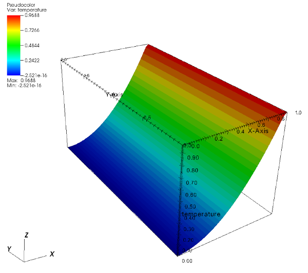
Domain is rectangular, its opposite corner coordinates being \((0,0,0)\) and \((1,2,2)\). We solve \(- \Delta T=f\) on the whole domain. 1D solution of the problem is set to \(x^p\). The right-end-side term \( f \) is equal to \(-p(p-1)x^{p-2}\). Figure 1 shows an illustration with \( p=2 \).

The global boundary conditions are chosen as follows.

Runtime parameters

Energy equation is used:

• temporal and inertial terms are disabled;
• MUMPS or HYPRE solvers can be used;
• linear or quadratic or cubic schemes for the boundary conditions are used.

Test cases

Files test_cases/verification/laplacian/dirichlet_3D_o2.nts and test_cases/verification/laplacian/dirichlet_3D_o4.nts are used to check the convergence as well as to verify the non-regression.

Comments

Since the problem is 1D, whatever the direction considered solutions should be equal up to computer precision. This is verified is the validation script of Notus on one mesh.

As regards to spatial convergence, when a centered second order scheme is used to discretize the Laplacian, we expect no error on the solution compared to the quadratic exact solution. This point is achieved only if a quadratic scheme is used to apply the boundary conditions (compared to a linear one).

Results

Second-order Laplacian

The case uses diffusion_scheme implicit o2_centered with bc_scheme linear. Second order convergence is observed with \(L_2\), \(L_1\) or \(L_\infty\) norms. The absolute error value is reduced when using quadratic boundary conditions.

Note

With bc_scheme quadratic former, the solution is reached up to computer precision whatever the mesh size.

Linear boundary conditions

Quadratic boundary conditions

Fourth-order Laplacian

For this case, we set the power of the solution to \( p=4 \).

The case uses diffusion_scheme implicit o4_centered with bc_scheme linear | quadratic | cubic.

For cubic, fourth order convergence rate of 4 is expected with \(L_2\), \(L_1\) or \(L_\infty\) norms.

A convergence study shows that the global order of accuracy is limited by the lowest-order component: second-order when linear extrapolation is used, third-order with quadratic, and fourth-order only when cubic extrapolation is applied at the boundaries.

Results

Linear boundary conditions

Second order convergence is achieved, limited by the lower-order boundary treatment.

Quadratic boundary conditions

Third order convergence is achieved, limited by the boundary treatment.

Cubic boundary conditions

Optimal fourth order convergence is achieved, thanks to the high-order boundary treatment.