vof-algebraic test case of single vortex (2D)

Description of the test case

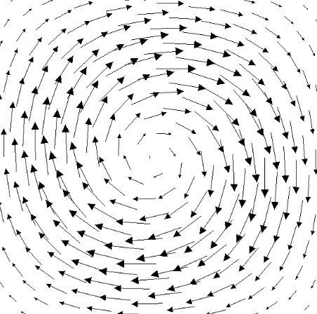
This test case solves advection of a disc of fluid in a sheared analytical velocity field. It is interesting because of the large variation of the interface topology. It is particularly adapted to measure mass-conservation. The objective is to verify the CICSAM advection scheme [1].

Configuration

Domain

The simulation takes place in a 2D box of coordinates \( (0,0) \) and \( (1,1) \). This domain is discretized uniformly with N cells in each directions. A bubble of fluid A is initialized in a domain full of fluid B. The coordinates of the center of the bubble at initial time is \( (0.5,0.75) \) with a \( 0.15m \) radius. The simulation runs during \( T=1.5s \).

Velocity field and time step

The velocity field is inverted at time \( t=T/2 \) such a way to obtain ideally a final state equal to the initial state.

Time t[s]	\(u(x,y)\)	\(v(x,y)\)
\( t<0.75s \)	\( 2sin^2(\pi x)cos(\pi y)sin(\pi y) \)	\(-2cos(\pi x)sin(\pi x)sin^2(\pi y)\)
\( t>0.75s \)	\( -2sin^2(\pi x)cos(\pi y)sin(\pi y) \)	\(2cos(\pi x)sin(\pi x)sin^2(\pi y)\)

Figure 1: Visualization of the velocity field, t>0.75s

To ensure that CFL of the method is always respected, we set a time step \( \Delta t \) such as

\begin{align} \Delta t = \frac{0.05}{N} \end{align}

Results

Evaluation of mass loss

In order to evaluate mass loss \( \varepsilon \) during the simulation, we compute the difference between the volume fraction of fluid at initial time and at time T.

\begin{align} \varepsilon = \sum \limits^{N^2}_{i=1}f_i - \sum \limits^{N^2}_{i=1} f_i^0 \end{align}

Mesh convergence evaluation

To evaluate mesh convergence, we define the \( L_1 \) norm of the difference between the initial and the current volume fraction as:

\begin{align} L_1 = \sum \limits^{N^3}_{i=1} |f_i - f^0_i| \\ \end{align}

We also compute local convergence order \( p \) of the method evaluating the evolution of the error with the mesh refinement:

\begin{align} p = \frac{ln\left( \frac{E_2}{E_1} \right)}{ln\left (\frac{N_1}{N_2} \right)} \end{align}

where \( E_1 \) and \(E_2 \) are error for mesh 1 and mesh 2, of size \( N_1\) and \(N_2\) respectively.

Results

The following tables show for different spatial discretization the material loss for the different advection methods.

\begin{align} cicsam method [1] \end{align}

Grid size N	\( \Delta x \)	\( \varepsilon_{air}\)	\( L_1 \)	p
16	1/16	\( -8.70 \times 10^{-6}\)	\( 2.87 \times 10^{-2}\)
32	1/32	\( -2.59 \times 10^{-5} \)	\( 7.30 \times 10^{-3}\)	\( 1.97 \)
64	1/64	\( -3.59 \times 10^{-5} \)	\( 2.32 \times 10^{-3}\)	\( 1.65 \)
128	1/128	\( -5.09 \times 10^{-5} \)	\( 1.21 \times 10^{-3}\)	\( 0.93 \)
256	1/256	\( -8.41 \times 10^{-5} \)	\( 6.44 \times 10^{-4}\)	\( 0.92 \)
512	1/512	\( -1.26 \times 10^{-4} \)	\( 3.51 \times 10^{-4}\)	\( 0.87 \)

\begin{align} mstacs method [2] \end{align}

Grid size N	\( \Delta x \)	\( \varepsilon_{air}\)	\( L_1 \)	p
16	1/16	\( -9.70 \times 10^{-6}\)	\( 3.54 \times 10^{-2}\)
32	1/32	\( -2.24 \times 10^{-5} \)	\( 8.15 \times 10^{-3}\)	\( 2.12 \)
64	1/64	\( -3.42 \times 10^{-5} \)	\( 2.10 \times 10^{-3}\)	\( 1.95 \)
128	1/128	\( -5.10 \times 10^{-5} \)	\( 9.00 \times 10^{-4}\)	\( 1.22 \)
256	1/256	\( -8.16 \times 10^{-5} \)	\( 4.68 \times 10^{-4}\)	\( 0.94 \)
512	1/512	\( -1.19 \times 10^{-4} \)	\( 2.41 \times 10^{-4}\)	\( 0.95 \)

\begin{align} stacs method [3] \end{align}

Grid size N	\( \Delta x \)	\( \varepsilon_{air}\)	\( L_1 \)	p
16	1/16	\( -5.02 \times 10^{-6}\)	\( 6.49 \times 10^{-2}\)
32	1/32	\( -1.78 \times 10^{-5} \)	\( 3.87 \times 10^{-2}\)	\( 0.74 \)
64	1/64	\( -3.20 \times 10^{-5} \)	\( 2.05 \times 10^{-2}\)	\( 0.92 \)
128	1/128	\( -5.11 \times 10^{-5} \)	\( 1.20 \times 10^{-2}\)	\( 0.77 \)
256	1/256	\( -8.14 \times 10^{-5} \)	\( 7.18 \times 10^{-3}\)	\( 0.74 \)
512	1/512	\( -1.02 \times 10^{-4} \)	\( 4.59 \times 10^{-3}\)	\( 0.64 \)

\begin{align} saish method [4] \end{align}

Grid size N	\( \Delta x \)	\( \varepsilon_{air}\)	\( L_1 \)	p
16	1/16	\( -1.01 \times 10^{-5}\)	\( 3.02 \times 10^{-3}\)
32	1/32	\( -2.44 \times 10^{-5} \)	\( 6.80 \times 10^{-3}\)	\( 2.15 \)
64	1/64	\( -3.65 \times 10^{-5} \)	\( 1.34 \times 10^{-3}\)	\( 2.33 \)
128	1/128	\( -5.26 \times 10^{-5} \)	\( 5.49 \times 10^{-4}\)	\( 1.29 \)
256	1/256	\( -8.57 \times 10^{-5} \)	\( 2.90 \times 10^{-4}\)	\( 0.92 \)
512	1/512	\( -1.26 \times 10^{-4} \)	\( 1.58 \times 10^{-4}\)	\( 0.87 \)

The results show that the method is not fully conservative. The different scheme has a first-order convergence and appears more stable when using a large number of cells.

References

[1] Ubbink, O., & Issa, R. (1999). A Method for Capturing Sharp Fluid Interfaces on Arbitrary Meshes. Journal of Computational Physics, 153(1), 26-50. https://doi.org/https://doi.org/10.1006/jcph.1999.6276 [2] Anghan, C., Bade, M. H., & Banerjee, J. (2021). A modified switching technique for advection and capturing of surfaces. Applied Mathematical Modelling, 92, 349-379. https://doi.org/https://doi.org/10.1016/j.apm.2020.10.038 [3] Darwish, M., & Moukalled, F. (2006). Convective Schemes for Capturing Interfaces of Free Surface Flows on Unstructured Grids. Numerical Heat Transfer, Part B : Fundamentals,49(1), 19-42. https://doi.org/10.1080/10407790500272137 [4] A. Arote, M. B., & Banerjee, J. (2021). An improved compressive volume of fluid scheme for capturing sharp interfaces using hybridization. Numerical Heat Transfer, Part B : Fundamentals, 79(1), 29-53. https://doi.org/10.1080/10407790.2020.1793543