|
|
0.6.0
|
|
|
0.6.0
|
Compressible steady natural convection benchmarks.
Compressible steady natural convection benchmarks.
Compressible flows can occur due to large temperature variations, resulting in large density changes for which the Boussinesq approximation and thus the incompressible assumption is no longer valid. The presebnt test-cases validate the proposed method [4] by reproducing the classical steady-state benchmarks "case T1" and "case T2" of [1]. From the nomenclature of [1], "case T1" refers to constant viscosity and conductivity while "case T2" refers to temperature-dependent viscosity and conductivity. The case considers Sutherland law for viscosity and conductivity (see section Configuration for parameters values).
We consider a differentially heated square cavity of length \(L\) subject to gravitational field \(\boldsymbol{g}\), filled with air considered as a perfect gas, with the following initial dimensionless parameters: temperature ratio \(\epsilon=\frac{T_{\mathrm{hot}}-T_{\mathrm{cold}}}{T_{\mathrm{hot}}+T_{\mathrm{cold}}}=0.6\), Rayleigh number \(\mathrm{Ra}_0=\mathrm{Pr}_0\frac{g\Delta T L^3 {\beta_p}_0\rho_0^2}{\mu_0^2}={1\times 10^{6}}\), Prandtl number \(\mathrm{Pr}_0 = {0.71}\). Initial Mach number (considering the characteristic velocity \(u_0=\frac{\lambda_0}{\rho_0 c_p L}\sqrt{\mathrm{Ra}_0}\)[2]) are \(\mathrm{Ma}_0 = {1.78\times 10^{-3}}\) for case T1 and \(\mathrm{Ma} = {1.81\times 10^{-3}}\) \(\mathrm{Ma}_0 = {2.15\times 10^{-3}}\) for case T2, respectively.
The boundary conditions of both cases are as follows. For temperature, the top and bottom walls are adiabatic conditions and left and right have respectively heated and cooled \(T_{\mathrm{hot}}=960\) K and \(T_{\mathrm{cold}}=240\) K. For velocity boundary conditions, all the boundaries have no-slip conditions. Both cases have been simulated considering an adaptative time step driven by an acoustic CFL=400. The implicit treatment of the pressure computation permits to consider large CFL number which amounts to naturally filtering acoustic waves.
We recall the Sutherland law for a material properties \(x\)
\[ x(T) = x^* \Big( \frac{T}{T^*} \Big)^{3/2} \frac{T^* + S}{T + S} \, , \]
with \(x^*\), \(T^*\) and \(S\) the three parameters of the law. For the present case, \(T^*=273\) \(S=110.5\), \(\mu^*=1.68\times 10^{-5}\) and \(\lambda^*=2.38\times 10^{-2}\)
The objective of the present validation is to compare the reference values of the spatial average side walls Nusselt numbers \(\overline{\mathrm{Nu}}_{\mathrm{left,right}}\) and cavity maximal pressure at steady state from[1] with our simulations. We propose a final time \(t_f=20\)s regarding the previous final time proposed [3] which verifies the steady state residuals of our simulations.
Main parameters to run this test case are:
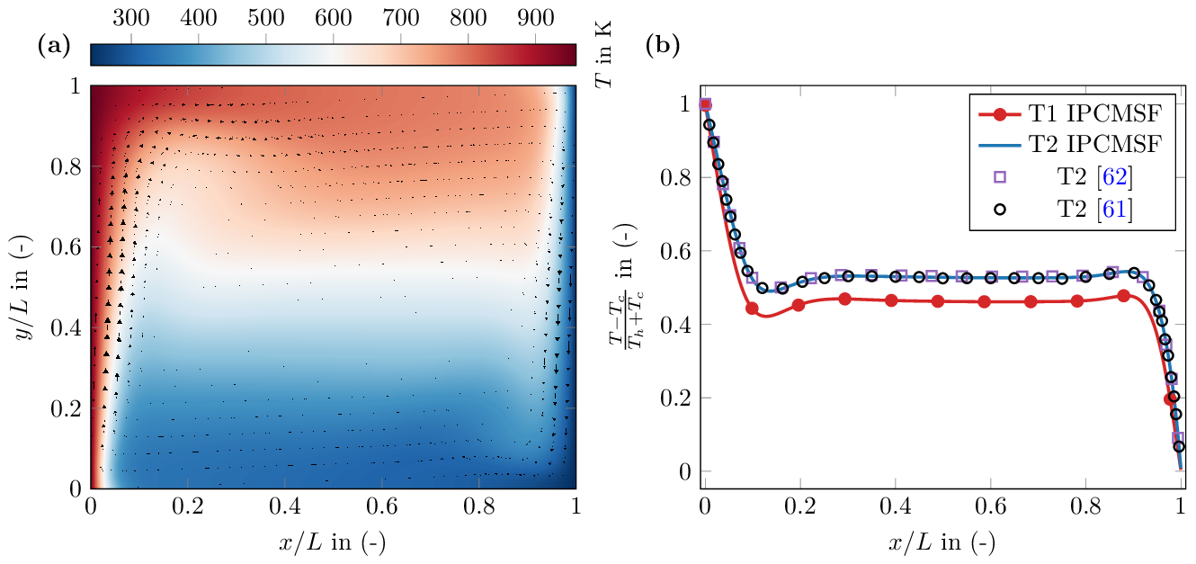
Figure 1 a,b presents respectively the pseudocolor plot of temperature field along with the velocity vectors field of the case T1 and the temperature profile comparison at $y=L/2$ between T1 and T2 cases. Simulation results of the T2 case [5,6] are also plotted in Fig.1b. The simulation of case T2 with our full compressible modelling well reproduces the temperature profile solution [5,6] while most of the benchmark contributions were obtained considering the low Mach number approximation [1,6]. To the author's knowledge, temperature profile solution of the case T1 is unavailable in the literature. We plot in Fig.1b this horizontal temperature profile and we validate this case in the following regarding Nusselt number and maximal pressure. As this configuration is simpler than T2, this approach is acceptable.
We propose in Table 1 a spatial convergence study of case T1 for regular meshes at \(\mathrm{CFL}=400\) also with Richardson extrapolated values. We observe a spatial second-order convergence on Nusselt numbers, spatial averaged pressure, temperature, and velocity.
Reference values of T1 are \(\bar{\mathrm{Nu}}={8.85978}\) and \(p_{\mathrm{max}}/p_0={0.856338}\)[1]. By carefully read the list of pitfalls and recommendations proposed by the authors of the benchmark [1], we verified the equality of the averaged left and right Nusselt number which for \(1024^2\) mesh are identical to three significant digits ( \(\overline{\mathrm{Nu}}_L - \overline{\mathrm{Nu}}_R = {9.48\times 10^{-5}}\)).
On the mesh size \(1024^2\), we found for the maximal pressure \(p_{\mathrm{max}}/p_0={0.855486}\). According to reference values[1], the absolute relative differences are respectively \({9.95\times 10^{-2}}\% \) for the maximal pressure and \({3.76\times 10^{-2}}\% \) for the Nusselt number (left value chosen).
| Mesh | Nusselt (left) | order | Nusselt (right) | order | Mean pressure | order |
|---|---|---|---|---|---|---|
| 64×64 | 9.05090157227307 | n/a | 9.08114728361273 | n/a | -17906.504680015983 | n/a |
| 128×128 | 8.911004038688283 | n/a | 8.91840496374799 | n/a | -15438.12219390235 | n/a |
| 256×256 | 8.871116131121639 | 1.810 | 8.872757641268556 | 1.834 | -14808.512415077188 | 1.971 |
| 512×512 | 8.859825956394248 | 1.821 | 8.860217909963438 | 1.864 | -14668.590951157334 | 2.170 |
| 1024×1024 | 8.85644726034052 | 1.741 | 8.856541989494461 | 1.770 | -14643.021905060044 | 2.452 |
| Extrapolation | 8.855004345874798 | n/a | 8.855017544586506 | n/a | -14637.304700904906 | n/a |
| Mesh | Mean velocity | order | Mean temperature | order |
|---|---|---|---|---|
| 64×64 | 0.049700033760768966 | n/a | 564.5339917012515 | n/a |
| 128×128 | 0.048601421383825456 | n/a | 568.229414716239 | n/a |
| 256×256 | 0.048313011993039605 | 1.929 | 569.2972156546181 | 1.791 |
| 512×512 | 0.048244647776091 | 2.077 | 569.5703002616473 | 1.967 |
| 1024×1024 | 0.04822959004370918 | 2.183 | 569.63881968148 | 1.995 |
| Extrapolation | 0.048225336615513245 | n/a | 569.6617703651156 | n/a |
Table 2 shows the spatial convergence study of case T2 for regular meshes at \(\mathrm{CFL}=400\) also with Richardson extrapolated values. Here, spatial second-order is observed on spatial averaged relative pressure, temperature and velocity, and varying between 1.63-1.85 for left and right Nusselt numbers. Reference values of this case are \(\overline{\mathrm{Nu}}=8.6866\) and \(p_{\mathrm{max}}/p_0={0.924487}\)[1]. On the mesh size \(1024^2\), we found for the maximal pressure \(p_{\mathrm{max}}/p_0={0.923744}\) and for the absolute difference between left and right Nusselt number \(1.4 \times 10^{-4}\). According to reference values[1], the relative differences are respectively \({7.4\times 10^{-4}} \% \) for the maximal pressure and \({7.8\times 10^{-4}} \% \) for the Nusselt number (left value chosen).
| Mesh | Nusselt (left) | order | Nusselt (right) | order | Mean pressure | order |
|---|---|---|---|---|---|---|
| 64×64 | 9.006734664685236 | n/a | 9.035028407543573 | n/a | -11447.76919098363 | n/a |
| 128×128 | 8.776653572035631 | n/a | 8.788137549233857 | n/a | -8973.03989780001 | n/a |
| 256×256 | 8.712926681898558 | 1.852 | 8.715505005029238 | 1.765 | -8006.941559023286 | 1.357 |
| 512×512 | 8.692388970506286 | 1.634 | 8.69297675213458 | 1.689 | -7771.454324988193 | 2.037 |
| 1024×1024 | 8.685817189944235 | 1.644 | 8.685957787230638 | 1.682 | -7726.864612433804 | 2.401 |
| Extrapolation | 8.682724785987721 | n/a | 8.682781247575674 | n/a | -7716.449377860505 | n/a |
| Mesh | Mean velocity | order | Mean temperature | order |
|---|---|---|---|---|
| 64×64 | 0.05689788742941662 | n/a | 599.5831240166381 | n/a |
| 128×128 | 0.05603685941715751 | n/a | 605.3753280536403 | n/a |
| 256×256 | 0.05568347256517695 | 1.285 | 607.4551251572764 | 1.478 |
| 512×512 | 0.05558533108820975 | 1.848 | 608.0775400649454 | 1.740 |
| 1024×1024 | 0.055561782714575673 | 2.059 | 608.2505093619335 | 1.847 |
| Extrapolation | 0.05555434870424454 | n/a | 608.3170766550376 | n/a |
[1] P. Le Quéré, C. Weisman, H. Paillère, J. Vierendeels, E. Dick, R. Becker, M. Braack, and J. Locke, Modelling of natural convection flows with large temperature differences: A benchmark problem for low mach number solvers. Part 1. Reference solutions, ESAIM: Mathematical Modelling and Numerical Analysis, 39(3):609–616, 2005. doi: 10.1051/m2an:2005027
[2] P. Le Quéré. Accurate solutions to the square thermally driven cavity at high rayleigh number. Computers & Fluids, 20(1):29–41, 1991. ISSN 0045-7930. doi: 10.1016/0045-7930(91)90025-d.
[3] A. Urbano, M. Bibal, and S. Tanguy. A semi implicit compressible solver for two-phase flows of real fluids. Journal of Computational Physics, 456:111034, 2022.
[4] J. Jansen, S. Glockner, D. Sharma, A. Erriguible, Incremental pressure correction method for subsonic compressible flows, Submited to Journal of Computational Physics, 2024.
[5] J. Vierendeels, B. Merci, and E. Dick. Benchmark solutions for the natural convective heat transfer problem in a square cavity with large horizontal temperature differences. International Journal of Numerical Methods for Heat & Fluid Flow, 13(8):10571078, 2003, doi: 10.1108/09615530310501957
[6] T. W. I. Kuan and J. Szmelter. A numerical framework for low-speed flows with large thermal variations. Computers & Fluids, 265:105989, 2023. ISSN 0045-7930. doi: https://doi.org/10. 1016/j.compfluid.2023.105989