Linear acoustic pulse propagation.

This test case investigates the isothermal problem of a linear acoustic wave propagation considering an inviscid perfect gas fluid ( \(\mu=0\)) with its equation of state

\[ \Delta p = c_0^2 \Delta \rho, \]

with \(\Delta p\) the pressure perturbation, \(\Delta \rho\) the density perturbation and \(c_0=\sqrt{\gamma R T_0}\) the constant speed of sound of the medium. This benchmark has been used in the past to test several novel compressible solvers [1,2,3,4,5,6] often to carry out temporal convergence studies. Besides its simplicity and the existence of analytical solutions, this case allows a clear evaluation of the numerical diffusion and dispersion of the proposed numerical schemes.

Configurations

We consider a monodimensional periodic domain of length \(L=1m\). For velocity boundary conditions, left and right boundaries have periodic conditions while top and bottom have slip conditions. At initial time, we consider the thermodynamic state \((T_0,p_0,\rho_0)=(300K,10^5Pa, \frac{p_0}{R T_0})\) and a Gaussian acoustic pressure wave defined as

\[ p(x,t_0) = p_0 + \Delta p_0 \exp(-\frac{x^2}{2\Sigma^2}), \]

with \(\Delta p_0\) the pulse amplitude and \(\Sigma\) a pulse length control parameter. The initial parameter of the pulse is set to \(\Delta p_0=10^2Pa\) and \(\Sigma=0.1m\) like in [5]. The dimensionless parameters of the problem are respectively \(\mathrm{Re}_0 = \infty\) and \(\mathrm{Ma}_0 = 7.14 \ 10^{4}\).

From the resolution of the d'Alembert equation, analytical solutions are available for all fields. The pressure, density and velocity solutions are respectively

\[ p(x,t) = p_0 + \Delta p_0 \exp\left(-\frac{\left(x-c_0 t\right)^2}{2\Sigma^2}\right)\, , \]

\[ \rho(x,t) = \rho_0 + \frac{\Delta p_0}{c_0^2} \exp\left(-\frac{\left(x-c_0 t\right)^2}{2\Sigma^2}\right), \]

\[ u(x,t) = \frac{\Delta p_0}{\rho_0 c_0^2} \exp\left(-\frac{\left(x-c_0 t\right)^2}{2\Sigma^2}\right), \]

with \(c_0 t\) the distance travelled by the wave.

Runtime parameters

Main parameters to run this test case are:

advection term of the Navier-Stokes equations not activated (Stokes flow)
incremental pressure correction method for subsonic compressible flows
BDF2 second order temporal scheme
implicit second order scheme
HYPRE or MUMPS solvers

Results

Next figure (a) presents a graphical temporal convergence study of the relative pressure field at \(t_f=c_0/L=2.88 \ 10{-3}s\) (time travelled by the wave until it returns to its initial position) for various acoustic Courant number, noted \(CFL\). The implicit treatment of pressure increment avoids a stability limitation related to acoustic time step as we do not find any stability limit (still stable at \(CFL=4000\), data not shown). For very large \(CFL\) and Euler backward temporal scheme, the acoustic wave is totally diffused but, note that for \(CFL=4,8\) the wave is still well predicted. We observe the relative low diffusivity of the first-order temporal scheme Euler backward at \(CFL=4\) compared to literature results [5] which obtain similar value of the maximum of the relative pressure with a low Courant number value (see \(CFL=0.5\) numerized curve from [5]).

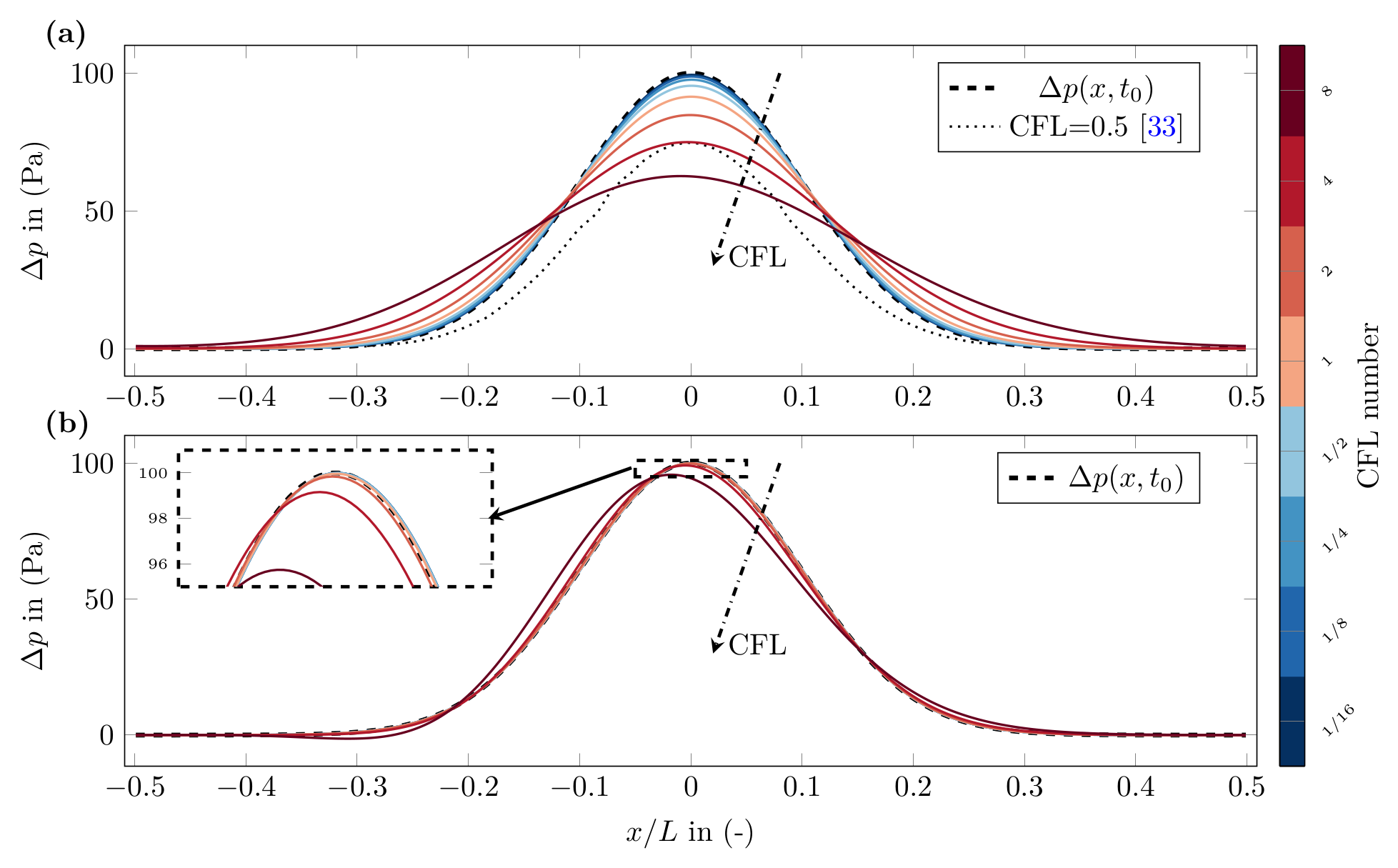
Figure 1: Acoustic pressure field variation at initial state t = 0 s (dashed line) and at tf = 2.88×10−3 s for various CFL (solid line colored by CFL value). (a) Euler backward temporal scheme. (b) BDF2 temporal scheme. Mesh size 512x8.

Additionally, it is noteworthy, on part (b) of the figure, that the BDF2 scheme, with second-order temporal accuracy, exhibits significantly lower numerical diffusion compared to the Euler scheme. This results in a pressure profile that closely aligns with the exact solution at \(CFL=2\). An error of less than \(1\%\) is observed compared to \(20\%\) with the Euler scheme. Using the BDF2 temporal scheme, the correct observation of acoustic propagation is possible while considering CFLs greater than unity.

In next tables, the temporal convergence study of this test case with the BDF2 scheme is presented with a final time \(t_f=L/c_s=2.88 \ 10^{-3}s\) and \(CFL=1\). First time step \(\Delta t=1.6 \ 10{-4}s\) is equal to \(CFL=2.84 \ 10^1\), mesh size is equal to \(512\!\times\!8\). Second-order temporal convergence is confirmed for pressure, velocity, and density, for both \(L_2\) and \(L_{\infty}\) norms.

Time step	Velocity L2 error	order	Velocity Linf error	order	Pressure L2 error	order
0.00016	0.04567511308746726	n/a	0.0969756971167619	n/a	18.419648481125442	n/a
8e-05	0.023040661811725035	0.987	0.05057052643421424	0.939	9.293373561480465	0.987
4e-05	0.007871063433196804	1.550	0.018461110879957804	1.454	3.1759544842508736	1.549
2e-05	0.0019860108340821712	1.987	0.00487317551443972	1.922	0.8016586080749134	1.986
1e-05	0.0003272307423698701	2.601	0.000751036560505236	2.698	0.13213976985276946	2.601

Time step	Pressure Linf error	order	Density L2 error	order	Density Linf error	order
0.00016	39.11237912552973	n/a	0.0001528094282489174	n/a	0.00032447634914145596	n/a
8e-05	20.392212028557736	0.940	7.70978394016906e-05	0.987	0.0001691738180567004	0.940
4e-05	7.451325473659168	1.452	2.634772261698379e-05	1.549	6.181620602019322e-05	1.452
2e-05	1.9683879274100207	1.920	6.6505608766816416e-06	1.986	1.632974885845684e-05	1.920
1e-05	0.3036241892607592	2.697	1.0962317060940545e-06	2.601	2.518866677236886e-06	2.697

We also present in the following tables the spatial convergence study with a constant Courant number \(CFL=1\). Second-order spatial convergence is confirmed for all fields considering both \(L_2\) and \(L_{\infty}\) norms.

Mesh	Velocity L2 error	order	Velocity Linf error	order	Pressure L2 error	order
16x8	0.05723446001301031	n/a	0.11153910125292044	n/a	23.083228485728153	n/a
32x8	0.030400313571282714	0.913	0.0684876275500017	0.704	12.263219838851635	0.913
64x8	0.010888678907157954	1.481	0.02650116841507552	1.370	4.394197978233194	1.488
128x8	0.0028515391729985223	1.933	0.006872393102497265	1.947	1.1511817510580113	1.933
256x8	0.0005231376899341912	2.446	0.0011813028362184785	2.540	0.2112741914471085	2.444
512x8	0.00013816071940312186	1.921	0.000283153575332179	2.061	0.05567420256992179	1.922

Mesh	Pressure Linf error	order	Density L2 error	order	Density Linf error	order
16x8	43.78283440304564	n/a	0.00019149849415735966	n/a	0.0003632224523231198	n/a
32x8	28.04361310572598	0.643	0.00010173568806080976	0.913	0.00023264985154902718	0.643
64x8	10.671073267337768	1.394	3.645427226010089e-05	1.481	8.852723799002149e-05	1.394
128x8	2.767924371417621	1.947	9.550205334804935e-06	1.932	2.296270425938829e-05	1.947
256x8	0.47675153113753765	2.537	1.7527309726821905e-06	2.446	3.955131335109385e-06	2.537
512x8	0.11399844733234943	2.064	4.6187325841851364e-07	1.924	9.457312704075349e-07	2.064

References

[1] J. Jansen, S. Glockner, D. Sharma, A. Erriguible, Incremental pressure correction method for subsonic compressible flows, Submited to Journal of Computational Physics, 2024.

[2] C. Wall, C. D. Pierce, and P. Moin. A semi-implicit method for resolution of acoustic waves in low mach number flows. Journal of Computational Physics, 181(2):545563, 2002.

[3] Y. Cang and L. Wang. An improved fractional-step method on co-located unstructured meshes for weakly compressible flow simulations. Computers and Fluids, 253, 2023. 2022.105775.

[4] D. Fuster and S. Popinet. An all-mach method for the simulation of bubble dynamics problems in the presence of surface tension. Journal of Computational Physics, 374:752–768, 2018.

[5] A. Urbano, M. Bibal, and S. Tanguy. A semi implicit compressible solver for two-phase flows of real fluids. Journal of Computational Physics, 456:111034, 2022.

[6] V. Moureau, C. Bérat, and H. Pitsch. An efficient semi-implicit compressible solver for large-eddy simulations. Journal of Computational Physics, 226(2):1256–1270, 2007. ISSN 0021-9991.