|
|
0.6.0
|
|
|
0.6.0
|
Immersed boundary compressible steady natural convection.
Immersed boundary compressible steady natural convection.
Natural convection in a cavity induced by an immersed heating body is considered in this section. The steady test case from[1] is considered with the following dimensionless parameters \(\mathrm{Ra}_0 = 5\times 10^{6}\), \(\mathrm{Re}_0 = 2.65\times 10^{3}\), \(\mathrm{Ma}_0 = 1.53\times 10^{-3}\), \(\mathrm{Pr}_0 = 7.1\times 10^{-1}\), \(\varepsilon=0.2\) with the reference velocity computed as \(V_0=\frac{\mu_0}{\rho_0 L}\sqrt{\mathrm{Ra}_0} \)[1]. We refer the reader to the original paper[1] for the geometrical configuration. The fluid filling the square cavity is air with variable Sutherland law for viscosity and conductivity. For the present case, \(T^*=273\) \(S=110.5\), \(\mu^*\)=1.68e-5 and \(\lambda^*=2.38\times 10^{-2}\). We propose for our simulations an acoustic CFL=400 and a final time \(t_f=30\){s} which verifies the steady state residuals of our simulations. A spatial first-order volume-penalty method is used [2]
The objective of the present validation is to compare the reference temperature and velocity profiles. We propose reference values of the spatial average side isothermal walls Nusselt numbers \(\overline{\mathrm{Nu}}_{\mathrm{left,right}}\) and cavity maximal pressure at steady state. We propose a final time \(t_f=30\){s} which verifies the steady state residuals of our simulations.
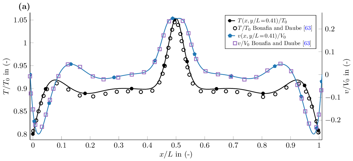
Figure 1a,b presents respectively horizontal profiles of dimensionless velocity and temperature and the pseudocolor plot of temperature field and velocity vectors field at the steady state. The characteristic flow described by[1], under a low Mach numerical method, is exactly found back by our simulations with the two counter-rotating recirculation zones cut off by a central plume induced by the heated immersed boundary (see Figure 1b). More importantly, the flow symmetry along the central vertical axis at this Rayleigh number is observed in Fig 1a,b. A discrepancy is visible for both velocity and temperature horizontal profiles (Figure 1a) between the literature data[1] and our simulation on the mesh $1024^2$. We report our $1024^2$ mesh as spatially converged and we note that Bouafia's data are very close to those produced by our $512^2$ mesh (data not shown).
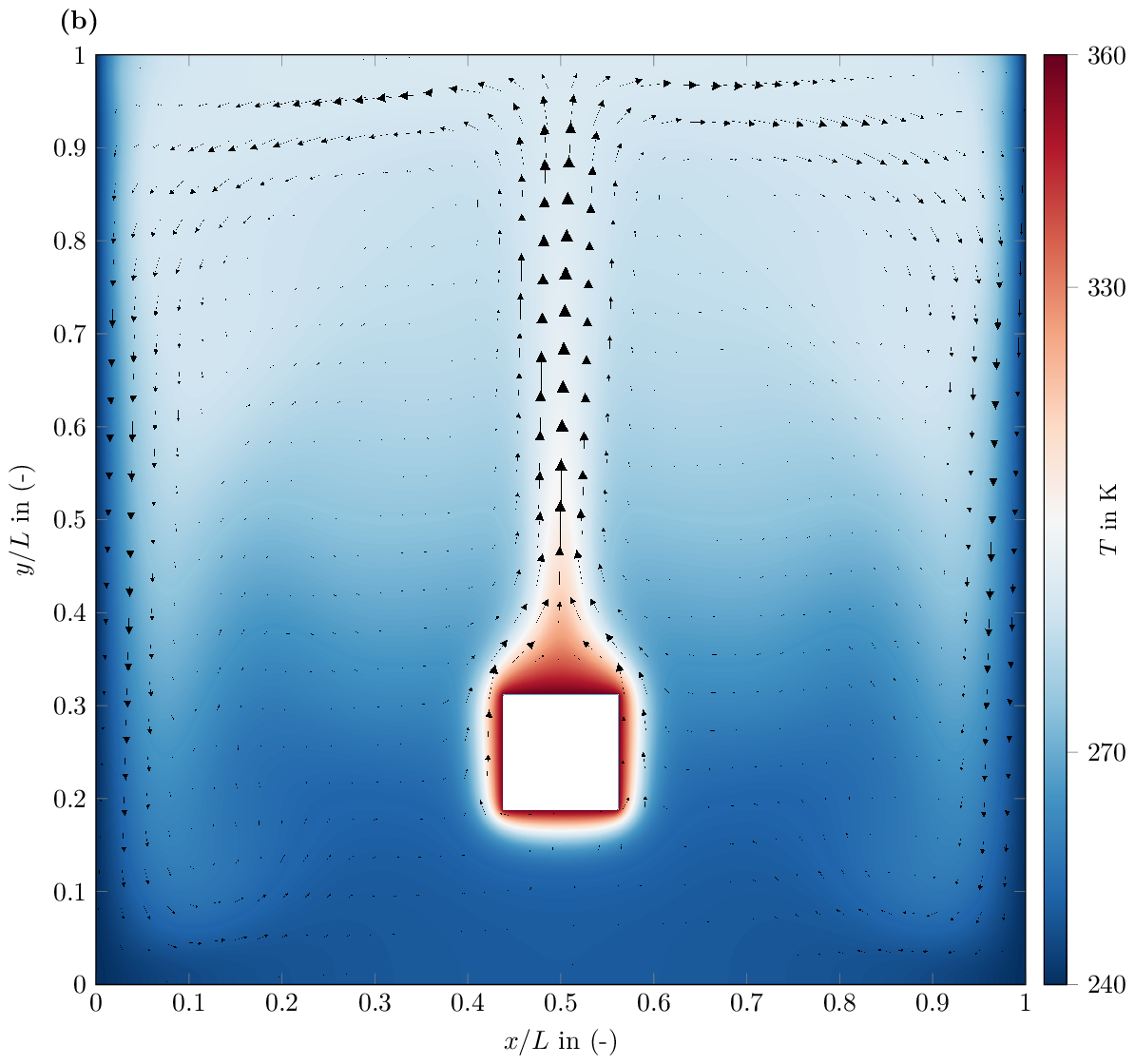
As expected due to the immersed boundary method used, first convergence order is observed (Table 1) on averaged Nusselt numbers, spatial averaged relative pressure, velocity, and temperature. Richardson extrapolated values are also provided in the table. To the author's knowledge, Nusselt numbers of this benchmark have never been reported, both on the side walls (Table 1), but also on the hot Immersed Boundary (IB), i.e. \(\mathrm{Nu}_{\mathrm{top}}^{\mathrm{IB}}={1.1681\times 10^{1}}\), \(\mathrm{Nu}_{\mathrm{bottom}}^{\mathrm{IB}}={3.0025\times 10^{1}}\), \(\mathrm{Nu}_{\mathrm{left}}^{\mathrm{IB}}={3.1641\times 10^{1}}\), \(\mathrm{Nu}_{\mathrm{right}}^{\mathrm{IB}}={3.1641\times 10^{1}}\) on the finest grid. For all Nusselt computations, we consider the length of the cavity as the characteristic length. The high Nusselt numbers of left, right, and bottom IB express the very thin thermal boundary layer observed compared to the top IB thermal boundary layer (see Fig 1b). Absolute difference between left and right Nusselt number for the entire cavity and for the immersed boundary are respectively \({1.41\times 10^{-4}}\) and \({1.2\times 10^{-11}}\).
| Mesh | Nusselt (left) | order | Nusselt (right) | order | Mean pressure |
|---|---|---|---|---|---|
| 64×64 | 6.1466841773118155 | n/a | 6.146684177311727 | n/a | -13616.993766465468 |
| 128×128 | 6.414504861366966 | n/a | 6.414504867661988 | n/a | -10792.825704128254 |
| 256×256 | 6.544248725265632 | 1.046 | 6.544248726125316 | 1.046 | -9926.301746057723 |
| 512×512 | 6.6136774052005265 | 0.902 | 6.613677405258415 | 0.902 | -9545.660977162197 |
| 1024×1024 | 6.650222122154842 | 0.926 | 6.65022212213761 | 0.926 | -9354.996735976363 |
| Extrapolation | 6.690835120596052 | n/a | 6.6908351213093225 | n/a | -9163.64229179723 |
| Mesh | order | Mean velocity | order | Mean temperature | order |
|---|---|---|---|---|---|
| 64×64 | n/a | 0.037090793174342856 | n/a | 269.6720190699074 | n/a |
| 128×128 | n/a | 0.03733820531219781 | n/a | 272.1852825042255 | n/a |
| 256×256 | 1.705 | 0.037498355221268355 | 0.627 | 273.21193313768714 | 1.292 |
| 512×512 | 1.187 | 0.03757191721001881 | 1.122 | 273.6596275499574 | 1.197 |
| 1024×1024 | 0.997 | 0.03760613035786564 | 1.104 | 273.87016376881695 | 1.088 |
| Extrapolation | n/a | 0.037635878107957085 | n/a | 274.0570664383566 | n/a |
[1] M. Bouafia and O. Daube. Natural convection for large temperature gradients around a square solid body within a rectangular cavity. International Journal of Heat and Mass Transfer, 50 (17–18):3599–3615, 2007. doi: 10.1016/j.ijheatmasstransfer.2006.05.013.
[2] K. Khadra, P. Angot, S. Parneix, and J.-P. Caltagirone. Fictitious domain approach for numerical modelling of navierstokes equations. International Journal for Numerical Methods in Fluids, 34 (8):651–684, 2000