Validation of the 2D turbulent heated flat plate flow with RANS standard and SST version of k-omega model.

This test case simulates the 2D incompressible turbulent flow over a heated flat plate with uniform constant wall temperature with RANS model (Reynolds-Average Navier-Stokes) \( k-\omega \). Without considering the gravity field and Boussinesq approximation, the energy equation is considered as a passive scalar in the present test-case. The well-documented configuration of the benchmark from NASA [1], a 2D zero-pressure-gradient flat plate of length \( L = 2 \) m, is used. We consider a uniform constant wall temperature plate of \( T_{\mathrm{wall}}=317\)K, corresponding to \( \Delta T = T_{\mathrm{wall}} - T_0 = 17 \) K.

Dimensionless number values are for Reynolds number based on half plate length \(\mathrm{Re}= u_{\infty} (L/2) / \nu = 5\cdot 10^{6}\), for Mach number \(\mathrm{Ma}=u_{\infty} / c_s =0.2\), for Prandtl number \(\mathrm{Pr} = c_p \mu / \lambda = 0.71 \). A unity fluid (air) is used with density \( \rho_{\infty} = \) 1 \( kg/m^3 \), kinematic viscosity \( \nu = u_{\infty}(L/2) /\mathrm{Re} = 1.39 \cdot 10^{-5} \), specific heat capacity at constant pressure \(c_p= 1004.5 \) J/kg/K and conductivity \( \lambda = \mu c_p / \mathrm{Pr} = 1.96 \cdot 10^{-2}\) W/m/K.

The freestream conditions for velocity, temperature, turbulent kinetic energy and specific dissipation rate are the same as in [1]: \( u_{\infty} = 69.26 \) m/s, \( k_{\infty} = 1.08 \cdot 10^{-3} m^2/s^2\) and \( \omega_{\infty} = 8.68 \cdot 10^{3} \) 1/s. We impose a constant freestream temperature at the inlet \( T_{\infty} = 300 \) K.

We validate Notus results of the implementation of standard k- \(\omega \) (labeled STD) [3] and SST k- \(\omega \) (labeled SST) [4] against correlations from Lienhard [5] and Reynolds et al., 1958 [6] in term of Nusselt number along the plate. The present validation ensures the accuracy and the reliability of the turbulence k- \(\omega \) models implemented in Notus when a passive scalar is coupled with RANS models.

Configurations

The boundary conditions are chosen as follows:

\( (u,v) \) :

Boundary	Condition	Value
left	inlet	\( (u_{\mathrm{\infty}}= 69.4,0) \)
right	Neumann
top	Slip
bottom PlateOffset	Slip
bottom Plate	Wall

\( T \) :

Boundary	Condition	Value
left	Dirichlet	\( T_{\infty}= 300 \)K
right	Neumann
top	Neumann
bottom PlateOffset	Neumann
bottom Plate	Wall

\( k \) :

Boundary	Condition	Value
left	inlet	\( k_{\mathrm{\infty}}= 1.08 \cdot 10^{-3} \)
right /top	Neumann
bottom PlateOffset	Neumann
bottom Plate	Wall

\( \omega \) :

Boundary	Condition	Value
left	inlet	\( \omega_{\mathrm{\infty}}= 8.68 \cdot 10^3 \)
right /top	Neumann
bottom PlateOffset	Neumann
bottom Plate	Dirichlet	\( \omega_{\mathrm{wall}}= 4.44 \cdot 10^{10} \)

The initial conditions are chosen as follows:

\( k_0 = k_{\mathrm{\infty}} \) : \( \omega = \omega_{\mathrm{\infty}} \), \( (u_0,v_0) = (u_{\mathrm{\infty}},0) \), \( T_0 = 300 \) K.

Mesh grid

Results are presented on the converged grid 707x384 proposed for the isotherm case with a composite mesh refinement. Along the vertical axis, two exponential meshes with different factors are applied. The first cell has \( \Delta y = 5 \cdot 10^{-7} \) m at the wall. Along the horizontal axis, the domain is divided into four zones:

The first zone, located before the leading edge, features a coarser exponential mesh.
The second zone, near the leading edge, is finely discretised with a uniform mesh.
The third zone is a transitional area with an exponential mesh extending to the midpoint of the plate.
Lastly, the fourth zone applies a coarser uniform mesh over the remaining half of the plate.

Runtime parameters

Main parameters to run this test case are:

Incremental pressure correction method for incompressible flows
BDF2 second order temporal scheme
HYPRE with boomeramg preconditioner for momentum, smg preconditioner for pressure, k and omega

Simulations stop when velocity stationnary reached a absolute tolerance of \(1 \cdot 10^{-6}\).

Comments

Turbulent Prandtl number of 0.9 is used to model the turbulent conductivity.

Results

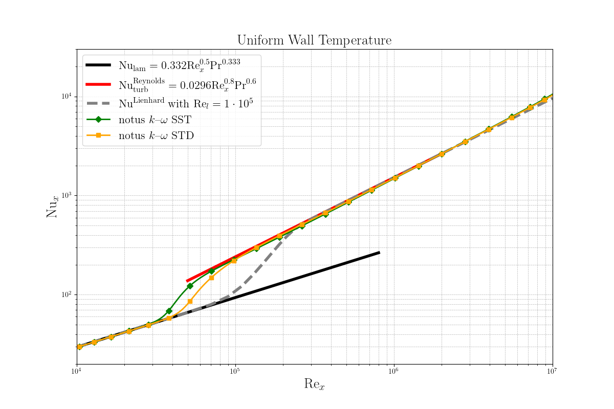
We validate the case by plotting in Figure 1 the Nusselt number variation along the plate \( \mathrm{Nu}_x = h_x x / \lambda \), with \( h_x = q_\mathrm{wall} / \Delta T\) and \( q_\mathrm{wall} = -\lambda_\mathrm{wall} \partial T/\partial y_\mathrm{wall}\). The results align well with the laminar and turbulent correlations from [5,6]. No deviations in \( \mathrm{Nu}_x \) are seen in both laminar and turbulent region for the k- \(\omega \) SST and STD versions while the transitional Reynolds number is different between STD and SST models.

Figure 2.a:

References

[1] NASA, 2D Zero Pressure Gradient Flat Plate Verification Case, Wilcox2006-klim-m Expected Results, https://turbmodels.larc.nasa.gov/flatplate_w06.html

[2] F. White (2011). Fluid Mechanics. New York City, NY: McGraw-Hill. pp. 477–478.

[3] D. C., Wilcox. Formulation of the k-w Turbulence Model Revisited. AIAA Journal, (46):2823–2838, 2008

[4] F. R. Menter. Two-equation eddy-viscosity turbulence models for engineering applications. AIAA Journal, 32(8):1598–1605, 1994

[5] J.H. Lienhard. Heat Transfer in Flat-Plate Boundary Layers: A Correlation for Laminar, Transitional, and Turbulent Flow. Journal of Heat Transfer, 2020.

[6] W. C. Reynolds, W. M. Kays, and S. J. Kline. Heat Transfer in the Incompressible Turbulent Boundary Layer: I—Constant Wall Temperature. 1958. NASA, Washington, DC, Memorandum