Compressible unsteady natural convection benchmark.

The last validation benchmark testing our method [3] is a recently proposed unsteady differentially heated square cavity with large temperature variations problem [1]. A two-dimensional cavity is filled with a perfect gas fluid with variable viscosity and conductivity following Sutherland law. For the present case, \(T^*=273\) K, \(S=110.5\), \(\mu^*\)=2.96e2 and \(\lambda^*\)=2.30E-01

Configurations

The dimensionless parameters of the reproduced benchmark are \(\mathrm{Ra}_0 =1.83e8\), \(\mathrm{Re}_0 = 1.61e4\), \(\mathrm{Ma}_0 = 1e-1\) (considering the reference velocity \(u_0=\sqrt{2\varepsilon L g}\) [1]), \(\mathrm{Pr}_0 = 7.1e-1\), \(\varepsilon = 0.6\). One can observe significantly larger Mach number compared to the [2] benchmark (ses cases T1 and T2 of compressible steady natural convection), providing an interesting complementary validation test case for subsonic compressible methods.

Boundary conditions are nearly identical as in . We introduce time-dependent hot and cold temperature boundary conditions

\[ T_L(t) = \frac{T_0+T_{L}^\infty}{2} + \frac{T_0-T_{L}^\infty}{2} \tanh(f_0(t - t_0/2) \, , \\ T_R(t) = \frac{T_0+T_{R}^\infty}{2} + \frac{T_0-T_{R}^\infty}{2} \tanh(f_0(t - t_0/2) \, , \]

with \(f_0=4/t_0\) 1/s and \(t_0=60\) s. \(T_{L,R}(t)\) tend to \(T_{L}^\infty=960\) K and \(T_{R}^\infty=240\) K, respectively. The proposed time-dependent Dirichlet conditions \(T_L(t)\) and \(T_R(t)\) allow avoiding the stiff initialization during the first iterations of BDF2 simulations. The reported BDF2 stiffness of the constant left/right temperature boundary conditions leads to the divergence of the simulation appearing at the very first iterations. This diverging feature has not been observed with Euler backward temporal scheme due to the diffusion of the scheme. We do not report any difference that is induced by the temperature ramps on the periodically established flow solution.

Unlike the benchamrks from [2] cases, comparative results on regular and Chebychev mesh grids point out the necessity of Chebyshev grid refinement to well capture the very thin boundary layer of the test case (see Figure 1a,b). We present in the following results on a \(256^2\) Chebyshev refined mesh with an adaptative time step driven by an acoustic CFL=2.5e3.

For an ease of reproducibility, we report our statistic start time \(t_s/t_{\mathrm{eddy}}=40\) and the end time \(t_f/t_{\mathrm{eddy}}=100\) of the simulation, with \(t_{\mathrm{eddy}}=4 L/(3 u_0)\) [1]. As performed by [1], we obtained a periodically established flow at this final time with relevant statistics of the resolved fields.

Objective

From data given by [1], the validation of this test case is achieved by the comparison of (a) the dimensionless temperature and velocity fluctuations spectrums, (b) the left and right time-averaged Nusselt number.

Runtime parameters

Main parameters to run this test case are:

incremental pressure correction method for subsonic compressible flows
BDF2 second order temporal scheme
HYPRE or MUMPS solvers

Results

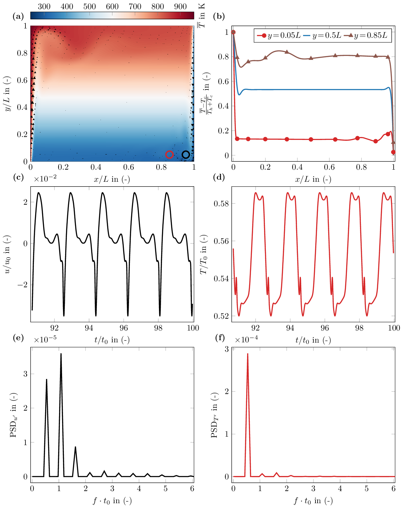
Figure 1a show the pseudocolor plot of the time averaged temperature and the velocity vector field at final time. In addition of the global overview of this natural convection benchmark and in order to provide reproducible data, we propose in Fig 1b three horizontal time averaged temperature profiles at final time along the vertical axis at \(y=0.05 L\), \(y=0.5 L\), \(y=0.85 L\), respectively.

Figure 1c,d show the time evolution of the instantaneous dimensionless velocity and temperature along the last five cycle. The localisation of the probes are for the temperature and velocity at \((x=0.85L,y=0.05L)\) and \((x=0.95L,y=0.05L)\), respectively. As found by [1], we find back two periodic signals of period \(T=1.85 t_{\mathrm{eddy}}\). Although we use a different numerical method, we observe an instantaneous temperature periodic temporal curve in good agreement with existing result [1]. Regarding the temporal evolution of instantaneous \(x\)-velocity (see Fig 1c), our temporal evolution during the period is relatively different from that reported although overall we find similar behavior. A possible reason is that we do not compare the temporal evolution of velocity at the same position in the cavity. In order to remove possible ambiguity on the location of the probes, we have marked them in Fig 1a.

We present in Figure 1e,f the Power Density Spectrum (PDS) of the dimensionless velocity and temperature fluctuations fields. The reported PDS [1] of a field \(x\) is computed as \(\mathrm{PDS}_x=|\widehat{x}|^2\) with \(\widehat{x}\) the Fast Fourier Transform (FFT) of \(x\). We thus compute the dimensionless PDS of the time-varying \(x\)-velocity fluctuation as \(\mathrm{PDS}_u(f) = |\widehat{u^\prime}|^2/u_0\), and temperature fluctuation \(\mathrm{PDS}_T(f)= |\widehat{T^\prime}|^2/T_0\). For both \(x\)-velocity and temperature fluctuations, we found the first five dimensionless frequencies \(\mathbf{f} \cdot t_{\mathrm{eddy}}=(5.4e-1, 1.0e0, 1.6e0, 2.2e0)^T\). Computed frequencies are consistent with reported values [1], e.g. the first frequency is in both studies \(f_1 t_{\mathrm{eddy}}\simeq 0.5\).

The left and right time-averaged Nusselts numbers computed on the last five cycles are respectively \(\overline{\mathrm{Nu}}_\mathrm{left}=34.73\), \(\overline{\mathrm{Nu}}_\mathrm{right}=34.66\). The absolute difference between left and right Nusselt is 7.44e-2. Our Nusselt numbers are consistent with the left reported value [1] of \(\overline{\mathrm{Nu}}_\mathrm{left}=34.2718\).

Figure 1: (a) Pseudocolor plot of time-averaged temperature field \(\overline{T}(x,y)\) and velocity vectors field at \(t_f=5.0051E+03\) s. (b) Horizontal time-averaged dimensionless temperature profiles at differents vertical positions and at \(t_f=5.0051E+03\) s. (c) Time evolution of the instantaneous dimensionless \(x\)-velocity \(u(x=0.95L,y=0.05L,t)/u_0\) during the last five periods. (d) Time evolution of the instantaneous dimensionless temperature \(T(x=0.85L,y=0.05L,t)/T_0\) during the last five periods. (e) Power density spectrum of the dimensionless \(x\)-velocity flucturation FFT. (f) Power density spectrum of the dimensionless temperature flucturation FFT. \(\mathrm{CFL}=2.5e3\), Chebyshev mesh size \(256^2\), \(t_f=100 t_\mathrm{eddy}=5.0051E+03\) s. The probes localisations for (c,e,d,f) plots are drawn on (a).

References

[1] X. Wen, L.-P. Wang, and Z. Guo. Development of unsteady natural convection in a square cavity under large temperature difference. Physics of Fluids, 33(8), 2021. doi: 10.1063/5.0058399.

[2] P. Le Quéré, C. Weisman, H. Paillère, J. Vierendeels, E. Dick, R. Becker, M. Braack, and J. Locke, Modelling of natural convection flows with large temperature differences: A benchmark problem for low mach number solvers. Part 1. Reference solutions, ESAIM: Mathematical Modelling and Numerical Analysis, 39(3):609–616, 2005. doi: 10.1051/m2an:2005027

[3] J. Jansen, S. Glockner, D. Sharma, A. Erriguible, Incremental pressure correction method for subsonic compressible flows, Submited to Journal of Computational Physics, 2024.