User-Defined Functions (UDFs)

Table of Contents

• Introduction
• Setting Up the Example Case
  • 1. Create the Directory Structure
  • 2. Define the Simulation Input File
  • 3. Create the Flow-Rate Post-Processing Utility
  • 4. Implementing the Post-Processing Utility
  • 5. Improving the Utility
  • 6. Exercise
• FAQ
  • Can I create a UDF library anywhere on the file system?
  • Can I use multiple UDF libraries simultaneously?
  • Why are UDFs in the test_cases directory compiled without the –udf option?

This guide explains how to create and use user-defined functions (UDFs) to extend the capabilities of the user interface beyond its default options.

Introduction

In some cases, the built-in tools provided by Notus may not offer enough flexibility to compute or initialize fields using custom logic or to perform advanced post-processing. User-defined functions (UDFs) offer a powerful and flexible mechanism for implementing such custom behavior within your CFD simulations.

Notus allows the creation of UDFs for various purposes such as post-processing, field initialization (e.g., initial conditions, source terms, linear terms), and defining custom equations. You can create multiple UDFs grouped into a UDF library.

This tutorial walks through the process of creating and integrating UDFs into your project.

To illustrate UDF usage, we will develop a post-processing utility to compute the flow rate through a cross-section in a 2D periodic Poiseuille flow (see Figure 1). This feature is not currently supported by the post_processing block of the user interface.

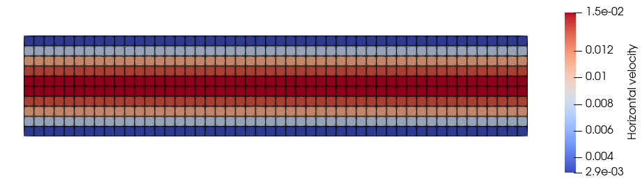
Figure 1: Periodic Poiseuille Flow

Setting Up the Example Case

Follow these steps to set up the simulation and demonstrate UDF functionality:

1. Create the Directory Structure

Create a tutorial directory at the root of the Notus project and add a poiseuille subdirectory:

mkdir -p tutorial/poiseuille
cd tutorial/poiseuille

2. Define the Simulation Input File

Create a file named poiseuille.nts in the poiseuille directory with the following content:

include std "physical_properties.nts";
 
double Height = 0.05;
double Length = 10*Height;
 
domain {
  spatial_dimension 2;
  corner_1_coordinates (0.0,   -Height);
  corner_2_coordinates (Length, Height);
 
  periodicity_x;
}
 
grid {
  grid_type regular;
  number_of_cells (50, 10);
  number_of_ghost_cells 2;
}
 
modeling {
  materials {
    fluid "water";
  }
 
  equations {
    navier_stokes {
      initial_condition {
        constant (0.0, 0.0);
      }
 
      boundary_condition {
        wall;
      }
 
      momentum_source_term {
        constant (1.2e-2, 0.0);
      }
    }
  }
}
 
numerical_parameters {
  time_iterations 100;
  time_step fixed 1e3;
 
  stop_tests {
    incompressibility 1e-11;
    stationarity_velocity 1e-11;
  }
 
  navier_stokes {
    time_order_discretization 1;
 
    boundary_condition_scheme quadratic;
 
    velocity_pressure_method rotational_incremental_pressure_correction;
 
    solver_momentum mumps_metis;
    solver_pressure mumps_metis;
  }
}
 
post_processing {
  output_library adios;
 
  output_frequency 10;
 
  output_fields velocity;
}

Ensure that Notus is compiled with MUMPS support (refer to How to Build Notus) and run the simulation:

mpirun -np 1 ./notus tutorial/poiseuille/poiseuille.nts

If successful, the simulation should converge by the 29th iteration, and the log will end with lines indicating convergence.

3. Create the Flow-Rate Post-Processing Utility

UDFs must be written in Fortran and stored in an out-of-tree directory (i.e., outside the src directory). To generate a UDF library, use the notus.py script with the add-udf tool. Run ./notus.py add-udf --help to view full documentation:

usage: notus.py add-udf [Options] UDF_NAME PATH
 
positional arguments:
  UDF_NAME              Identifier of the UDF library.
 
  PATH                  Path to the directory of the UDF library.
 
 
Options:
  -h, --help            show this help message and exit
 
  --all                 Enable all available UDFs.
 
  --preprocess          Enable UDF to perform custom setup before the time loop.
 
  --boundary-conditions
                        Enable UDF to set boundary conditions.
 
  --reference-solutions
                        Enable UDF to set reference solutions.
 
  --initial-conditions  Enable UDF to set initial conditions.
 
  --source-terms        Enable UDF to set source terms.
 
  --linear-terms        Enable UDF to set linear terms.
 
  --prepare             Enable UDF to prepare equations.
 
  --post-process        Enable UDF to do custom post-processing.
 
  --probe-fields        Enable UDF to probe custom fields.
 
  --material-properties
                        Enable UDF to set material properties.
 
  --pressure-update     Enable UDF to customize pressure update.
 
  --grad-div-coef       Enable UDF to set the grad-div operator coefficient.
 
  --checkpoint-restart  Enable UDF to perform checkpoint-restart.
 
  --user-equations      Enable UDF to setup user equations 'user_scalar' or 'user_vector'.
 
  --advection-scheme    Enable UDF to write a custom advection scheme.
 
  --diffusion-scheme    Enable UDF to write a custom diffusion scheme.
 
 
Example:
    $ ./notus.py add-udf --boundary-conditions flux tests/case/
    creates the 'test/case/udf_flux' directory

This utility requires two arguments:

• UDF_NAME: the name of the UDF library. Note: The resulting directory name will be prefixed with udf_, so specifying flow_rate will create a directory named udf_flow_rate.
• PATH: the directory where the UDF library will be created.

For post-processing, execute the following command from the Notus root directory:

./notus.py add-udf --post-process flow_rate tutorial/poiseuille

If successful, you will see output confirming that the UDF files were created and instructions to compile and use the library (last two lines):

Process UDF file: 'tools/udf_template/main.f90' → 'tutorial/poiseuille/udf_flow_rate/main.f90'
Process UDF file: 'tools/udf_template/CMakeLists.txt' → 'tutorial/poiseuille/udf_flow_rate/CMakeLists.txt'
Process UDF file: 'tools/udf_template/post_process.f90' → 'tutorial/poiseuille/udf_flow_rate/post_process.f90'
────────────────────────────────
Append '--udf tutorial/poiseuille/udf_flow_rate' to the ./build_notus.sh command
Add 'load_udf_library "udf_flow_rate/libflow_rate.so";' to the 'system' block of the NTS file.

The generated directory structure will be:

tutorial/
└── poiseuille
    ├── poiseuille.nts
    └── udf_flow_rate
        ├── CMakeLists.txt
        ├── main.f90
        └── post_process.f90

Edit main.f90 only if you need to add a UDF type that wasn't initially enabled. You can safely ignore this file most of the time. Your main implementation will go into post_process.f90.

To compile the library:

./build_notus.sh -a -j 64 --udf tutorial/poiseuille/udf_flow_rate

You should see output confirming that the build script have found the UDF library:

-- UDF libraries provided by user:
--   UDF directory: tutorial/poiseuille/udf_flow_rate

The resulting shared object file libflow_rate.so will be placed in the udf_flow_rate directory. To use it, add the following line to the poiseuille.nts file before the domain block:

system {
  load_udf_library "udf_flow_rate/libflow_rate.so";
}

Rerun the simulation:

mpirun -np 1 ./notus tutorial/poiseuille/poiseuille.nts

You should see output confirming that Notus loaded the UDF library:

Loading UDF library 'tutorial/poiseuille/udf_flow_rate/libflow_rate.so'
 Loaded UDF: post_process

Before proceeding, note that since the post_process.f90 file is still empty, there is no other visible effect yet. We now need to implement the logic to compute the flow rate.

4. Implementing the Post-Processing Utility

Edit the post_process() subroutine in post_process.f90 as follows:

subroutine post_process()
   use fields_navier, only: velocity
   use mod_notus_log, only: notus_log_double
   use variables_cell_spatial_steps, only: dy
   use variables_grid, only: js, je
 
   integer, parameter :: i = 27 ! Center of the domain
   integer, parameter :: k = 1  ! 2D case
   double precision :: flow_rate
   integer :: j
 
   flow_rate = 0d0
 
   do j = js, je
      flow_rate = flow_rate + velocity%u(i,j,k) * dy(j)
   end do
 
   call notus_log_double("Flow rate: ", flow_rate, 1)
end subroutine post_process

Recompile the UDF (no need to specify --udf again, unless you have used the clean option -c):

./build_notus.sh -S -j 64

Run the simulation again and look for Flow rate: messages in the log. At iteration 29, the flow rate should be approximately:

Flow rate: 1.00499999758205485E-003

The expected flow rate (per unit of depth) for a Poiseuille flow is:

\[ Q = \frac{2}{3}\frac{f h^3}{\nu} \]

Where:

• \( f \) is the momentum source term, which in our case is \(f=1.2\cdot 10^{−2} \mathrm{m\;s}^{-2}\),
• \( \nu \) is the kinematic viscosity of water, typically \(\nu=10^{−6} \mathrm{m}^2\mathrm{s}^{-1}\),
• \( h \) is the half-height of the channel, defined as Height = 0.05.

Substituting the values gives \( Q = 10^{-3}\mathrm{m^2}\mathrm{s}^{-1}\).

This result matches the numerical flow rate obtained from Notus.

Currently, the utility works for a single MPI process and uses a hard-coded x-position. In future sections, we will demonstrate how to make it parallel and more flexible.

5. Improving the Utility

To enhance flexibility and parallel execution, we will replace the hard-coded x-index of the cross-section with a user-defined variable.

a. Declaring a Configurable Cross-Section

First, define a variable named iCrossSection in the system block of your .nts file. This variable represents the x-index of the cross-section and will be exported so it can be accessed from the UDF:

system {
  integer iCrossSection = 20;
  export iCrossSection;
  load_udf_library "udf_flow_rate/libflow_rate.so";
}

You can declare and export variables anywhere in the .nts file, but placing them near the UDF loading directive helps with readability and organization.

b. Accessing Exported Variables

In Fortran, exported UI variables can be accessed using the variables_ui module. Depending on the variable type, use one of the following functions:

• ui_get_integer(name)
• ui_get_double(name)
• ui_get_boolean(name)
• ui_get_string(name)

For our example, we use ui_get_integer("iCrossSection") to retrieve the x-index.

c. Handling Parallel Execution

To ensure the utility works in parallel:

• Use variables_mpi to check whether the cross-section lies within the local domain. is_global_physical_domain and ie_global_physical_domain store the bounds of the local domain.
• Compute the local contribution only if the cross-section is inside the local domain.
• Use global_sum() to gather results from all MPI processes.

Update the post_process() subroutine as follows:

subroutine post_process()
   use fields_navier, only: velocity
   use mod_global_sum, only: global_sum
   use mod_notus_log, only: notus_log_double
   use variables_cell_spatial_steps, only: dy
   use variables_grid, only: is, js, je
   use variables_mpi, only: isg => is_global_physical_domain, &
      &                     ieg => ie_global_physical_domain
   use variables_ui, only: ui_get_integer
 
   integer, parameter :: k = 1  ! 2D case
   double precision :: flow_rate
   integer :: id, i, j
 
   ! Retrieve the cross-section index from the UI
   id = ui_get_integer("iCrossSection")
 
   flow_rate = 0d0
 
   ! Compute flow rate if the cross-section lies in the local domain
   if (id >= isg .and. id <= ieg) then
      ! Convert global index to local cell coordinate.
      i = isg - id + is
      do j = js, je
         flow_rate = flow_rate + velocity%u(i,j,k) * dy(j)
      end do
   end if
 
   ! Accumulate contributions across all MPI processes
   call global_sum(flow_rate)
 
   ! Print result to the Notus log
   call notus_log_double("Flow rate: ", flow_rate, 1)
end subroutine post_process

You can now run the simulation with multiple MPI processes. If you increase the number of processes, you may also need to increase the number of grid cells in the x-direction to ensure load balancing.

---

6. Exercise

Modify the utility so that the cross-section is defined by a physical x-coordinate rather than a cell index.

Goal

• Declare a double variable named xCrossSection instead of iCrossSection.
• Update the UDF to use this coordinate.
• Convert the x-coordinate to the nearest cell index or use linear interpolation.

Hints

• Use ui_get_double("xCrossSection") to retrieve the value.
• You can access cell coordinates with the variables_cell_coordinates module.
• Since the computation will use local coordinates, you no longer need variables_mpi.

---

FAQ

Can I create a UDF library anywhere on the file system?

Yes, as long as you provide the full path with the --udf option when building.

Can I use multiple UDF libraries simultaneously?

Yes, simply load multiple libraries in the system block of your .nts file:

system {
  load_udf_library "udf_utility_A/libutility_A.so";
  load_udf_library "udf_utility_B/libutility_B.so";
}

If both libraries implement the same UDF (e.g., post_process()), they will be called in the order in which they are loaded.

Why are UDFs in the test_cases directory compiled without the –udf option?

The build system (via CMake) automatically detects UDFs placed in certain subdirectories of test_cases. This helps streamline the build process for non-regression tests without requiring manual specification of each UDF path.