Kovasznay flow test case (2D)

This test case solves the 2D steady Kovasznay flow on a square domain at \( Re=40 \) (Reynolds number). Unlike the Poiseuille flow, the analytical solution is not polynomial (it involves exponential and trigonometric terms), so a second order centered scheme cannot represent it exactly: the discretization error is non-zero and decreases at the expected order. This makes the case a good verification of the actual spatial convergence order. The aims of this test case are:

validate the discretization of the steady Navier-Stokes equations on a non-trivial analytical solution.
verify the second order spatial convergence of the velocity in the \( L_1 \), \( L_2 \) and \( L_\infty \) norms.

Configurations

Domain is a unit square, its opposite corner coordinates being \( (0,0) \) and \( (L,L) \) with \( L=1 \). We solve the Navier-Stokes equations on the whole domain. The exact velocity is imposed on every boundary (full Dirichlet). The configuration is summarized in the next table.

Boundary	Condition	Value
left	Dirichlet	Exact Kovasznay velocity
right	Dirichlet	Exact Kovasznay velocity
bottom	Dirichlet	Exact Kovasznay velocity
top	Dirichlet	Exact Kovasznay velocity

Since the velocity is imposed on all boundaries, the pressure is only defined up to an additive constant; the pressure solver fixes the gauge internally.

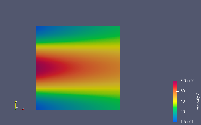
Figure 1: u velocity component of the Kovasznay flow

The exact (analytical) velocity field is:

\[ u(x,y) = U_{ref} \left( 1 - e^{\lambda x / L} \ \cos\left(\frac{2\pi y}{L}\right) \right) \]

\[ v(x,y) = U_{ref} \ \frac{\lambda}{2\pi} \ e^{\lambda x / L} \ \sin\left(\frac{2\pi y}{L}\right) \]

where the decay rate \( \lambda \) is:

\[ \lambda = \frac{Re}{2} - \sqrt{\frac{Re^2}{4} + 4\pi^2} \]

with \( Re=40 \), \( L=1 \) and \( U_{ref}=Re \).

Note: The fluid fluid_one has all physical properties set to 1 ( \( \rho=1 \), \( \mu=1 \), hence \( \nu=1 \)). The effective Reynolds number \( Re = U_{ref} L / \nu = 40 \) then matches the value used to build \( \lambda \), so the imposed field is indeed an exact solution of the Navier-Stokes equations.

Runtime parameters

Navier-Stokes equation is used:

the advection term is solved (implicit, \( o2\_centered \) scheme)
HYPRE or MUMPS solvers are used

Comments

Because the exact solution is exponential and trigonometric, it cannot be represented exactly by the second order centered scheme. A non-zero error is therefore expected on every mesh, decreasing at second order as the mesh is refined. This is the main difference with the Poiseuille flow, whose quadratic solution is captured up to computer precision.

Only the velocity is checked against a reference solution. The analytical pressure of the Kovasznay flow is known and could be added as a further verification.

Results

The grid size starts from 16 in every direction up to 128, with a geometric refinement factor of 2. Second order convergence is observed for the velocity in the \( L_1 \), \( L_2 \) and \( L_\infty \) norms on regular meshes.

2D results

mesh	\(L_1\) error	Order	\(L_2\) error	Order	\(L_\infty\) error	Order
16	1.882568e-01	n/a	1.962496e-01	n/a	4.128963e-01	n/a
32	4.756635e-02	1.985	4.892095e-02	2.004	1.148312e-01	1.846
64	1.187821e-02	2.002	1.229019e-02	1.993	3.505389e-02	1.712
128	2.969428e-03	2.000	3.079559e-03	1.997	9.820875e-03	1.836

The \( L_1 \) and \( L_2 \) norms converge cleanly at order 2. The \( L_\infty \) norm, dominated by the local error near the strongest gradients, also converges at order ~2 with the expected mild oscillation.

References [1] https://www.karlin.mff.cuni.cz/~prusv/teaching/2016-2017/zs/downloads/kovasznay.pdf