Project source organization

The following guidelines describes how project files are organized.

Top-level directory

The usage of each sub-directory is listed below:

Name	Description
doc	Doxygen generated documentation
logo	The Notus logo
src	Fortran source files
std	Standard database
test_cases	Test case description files
tools	Useful development and validation scripts

The src directory

The sources of Notus are devided into 4 parts:

1. The Notus library sources that are compiled first to create its library libnotus.a. Corresponding files are in src/lib.
2. The user interface, the main program and some specific routines associated to some test cases are compiled on a second step and linked with libnotus.a. They can be found in src/notus.
3. The doc sources in src/doc.
4. Some unit testing in src/unit_testing directory.

Architecture

The library architecture is based on 8 different modules that the developer will find in the corresponding source directories. The following section describes each module as well as its interaction with others.

Figure 3: Notus code architecture

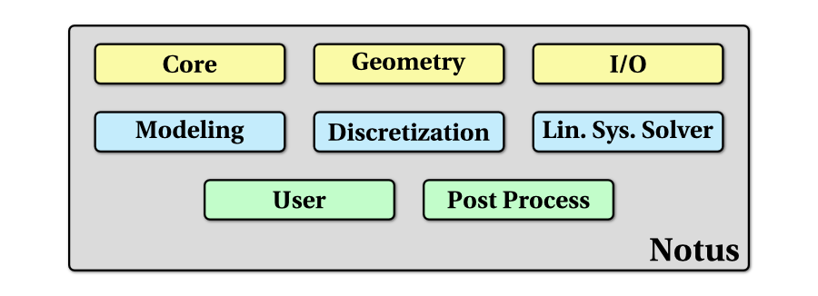
The src/lib directory

User module

The User module is the place where the advanced user can develop its own code when the NTS files aren't sufficient for his/her needs.

Core module

The Core module furnishes the base code on which is built the library. It contains the following sub-modules:

• system: the Notus dynamic execution procedures (memory allocation, performance monitors, etc.)
• data_structures: the face_field (for face-based vector fields), the boundary_conditions related structures and the containers (linked lists, maps, etc.) derivable types
• parallelism: parallel threads construction and data exchange procedures between processors
• misc: various useful functions, notably mathematical functions (constants, algebra, polynomial roots, etc.)

Modeling module

The Modeling module is the place where the equations of the physical models (see Brief description of models and equations) are solved. To do so, it uses principally the Discretization and the Linear System Solver modules. This is where the model developer will integrate his own code. We use high-level numerical methods term for this module.

The following sub-modules are furnished in the library and can serve as examples:

• navier: the incompressible Navier-Stokes equations
• energy: the energy (temperature) equation
• species_transport: the transport of one or multiple species by the flow
• turbulence: the turbulence models
• phase_advection: the advection of immiscible phases
• compute_physical_fields: is used for density and viscosity computation
• generic_transport_equation: is used by both the energy and the species_transport equations, as they share similarities in their solving

Discretization module

The Discretization module furnishes all the computation procedures and functions that are (mainly) used by the Modeling module to effectively solve the equations. For example, the developer will find there all the differential cell or face operator implicit discretization routines, the explicit differential operators (gradient, divergence, etc.) and finite difference schemes. We use the low-level numerical methods term for this module. The model developer will use this part of the library, whereas the numerical developer will develop his own methods inside it.

It is divided in sub-modules:

• implicit_discretization: the main implicit discretization methods for face or cell based terms
• explicit_discretization: the explicit discretization methods for face or cell based terms
• differential_operators: operators (gradient, divergence, laplacian, etc.) defined on cells and faces
• node_level_schemes: finite difference schemes, interpolation and extrapolation methods (for example, used by the above sub-modules)
• time: procedures for time related discretization questions
• immersed_boundary: particular discretization operations for the immersed boundaries
• multiphase: multiphase methods (VOF, MOF, level set)

Post process module

The Post process module furnishes all the tools that are used and can be used to extract numerical and physical diagnostics from the computed data. For example, one can use this module to compute the \(L_2\) norm of the error to a reference solution, or the strain rate based on the velocity field.

It is divided in sub-modules:

• error_computation: error computation on nodes and different norms ( \(L_2\), \(L_1\), \(L_\infty\))
• integration: integration useful functions (eg. compute the integral of a cell field)
• physical_diagnostic: a collection of physical based diagnostic quantities (vorticity, Nusselt number, etc.) that can be computed from the various fields
• validation: a place used to process validation related data (eg. particular output for grid convergence)

Geometry module

The Geometry module contains procedures related to the discrete and physical geometry of the problem. It is separated in two distinct sub-modules:

• grid: this is where the discrete grid is defined and constructed from the input physical boundaries. The developer will find there the important data structures (coordinates, spatial steps, etc.) and useful associated functions (eg. get the \((x,y,z)\) coordinates of a cell's center)
• computational_geometry: this module proposed a set of geometrical shape definition (eg. circle, square, etc.) that are used at initialization and useful functions to manipulated 3D meshes (with triangles, polygons, tetrahedrons)

Linear system solver module

The Linear system solver module handles the different solvers encapsulated into Notus and the external solver interfaces. It furnishes the procedure to use the three following solvers:

• hypre_interface: the HYPRE library Notus interface
• mumps_interface: the MUMPS library Notus interface
• notus_solver: the Notus internal solver

I/O module

The Input/Output module proposed the various procedures to read the input data and write output information and results. It contains also the log and debug procedures to display/save various information during the calculus.

It is divided in sub-modules:

• log: mainly the useful notus_log function for printing specific output during the calculations
• debug: functions to write debug output
• adios_interface: the interface between Notus data fields and Adios data procedures
• lexer_parser: procedures for the reading and parsing of the input file
• checkpoint_restart: procedures to export data (checkpoint) that can be used to start again a computation in case of a computer crash (restart)

For a complete view of this directory at a lower level, see Modules and topics on left menu. It contains numerical method and source descriptions.

The src/notus directory

The main program notus.f90 is found in src/notus directory. It is described next section (Code overview).

Routine finalize_initialization.f90 finalizes the initialization process of a simulation. It is called just before the time loop.

test_cases subdirectory

Fortran programs relative to some test cases that cannot be completely described by the User Interface are present in the test_cases subdirectory. For instance, it may be some time dependant velocity field, spatial dependant boundary conditions, etc. There is one subdirectory associated to the each test case that need such routines. In this case, a keyword is present in the corresponding NTS file. For instance:

test_case tc_vof_sheared;

These routines may be called to initialize, prepare next time loop iteration, or for post-processing purposes.

ui subdirectory

The user interface is in the ui sub-directory.

comand_line subdirectory

It contains routines that read Notus command line.

The src/doc directory

This directory contains doc sources (Markdown .md files) which are not directly linked to a source file but describe some basic concepts of the code (build, source organization, description of the domain, etc.).

The src/unit_testing directory

This directory contains the Unit Testing ('UT') subdirectories that are aimed to test and validate each individual element/part of the code, separately.

The test_cases directory

This directory contains the test cases NTS files that are used to verify and validate Notus. Verification analyzes the solution of the code when an exact solution of the problem exists (or is eventually manufactured). It is essentially a mathematical process. Validation checks the capacity of the code to represent a physical problem (flow, heat transfer, etc.) that do not have an exact solution.

Thus, the Notus test cases are divided into 2 groups, verification and validation test cases. Each test case is described by an NTS file that is read by the parser of Notus. It follows a specific succession of information (grammar) about the domain and the mesh, the modeling and the numerical methods, and finally about post-processing.

The description of each test case and their expected results can be found in these two pages verification and validation.

Enventually, some specific routines associated to initialization, time dependant source terms or boundary conditions, etc., are defined in src/notus/test_cases directory, that follows the same tree then then the test_cases directory.

The std directory

This directory contains the standard Notus database that is reduced at present time to the fluid physical properties database physical_properties.nts.